Analytical Prediction
By Hayden McLeod (hmcleod6)
Claimed/Edited by Lauren Widjaja (Fall 2018)
Deprecated by Richard Udall (Summer 2019), see Kinematics instead, some content may be spliced from here into that article
Using the momentum principle and a knowledge of the net force on an object, we can iterative calculations to predict the motion of that object over time. We have already seen how to do this with a constant net force, and will soon see how to do it with a varying force. However, if the force is constant, we may also solve the problem analytically, with no iteration necessary. Many non-constant forces may also be solved analytically, but this requires more complex mathematics.
The Main Idea
Analytic prediction is the process of producing a general formula for an objects motion over time. In contrast to iterative prediction, there is no need to perform calculations at regular intervals. However, the assumptions we will be making here only hold if the force is constant: non-constant forces demand the use of differential equations as a method of solution in all but the simplest cases. Due to this limitation, iterative prediction may be applied directly in a wider variety of situations, and may be used in cases where the forces are too complex to allow any analytic solution (see Determinism). However, analytic prediction may be used for many simpler cases, and in more complex cases may allow for estimation of values if a computer program is unavailable or prohibitively slow. One of the most prominent examples of the use of analytic modelling will be in solving Projectile Motion problems.
A Mathematical Model
Unlike the iterative prediction method which is derived directly from the momentum principle, the formula for analytical prediction is based of the formula for the arithmetic mean. Here, X bar is the arithmetic mean, sigma f x is the sum of all the values, and sigma f is the total number of terms. Since we only need two values of velocity to calculate the average velocity, the formula, for this purpose, can be simplified.


In addition, if Fnet is constant, we can derive the kinematic equations such as:
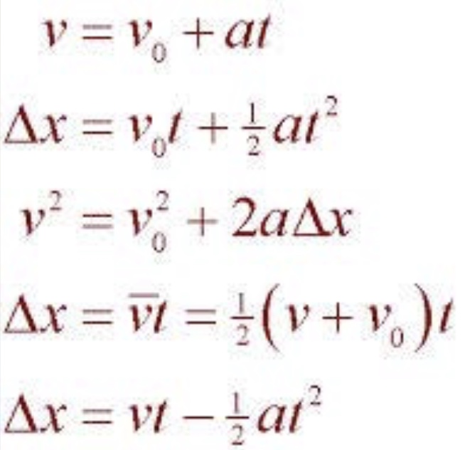

Projectile motion (neglecting air resistance) is a common example to illustrate the effects of a constant force. The equations are:
x(t) = (Vx,o)t +xo
y(t) = 1/2(-g)t^2 + (vy, o)t + yo
A Computational Model
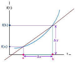
Below is a visualization of the analytical prediction of the average velocity. As you can see, it takes two points, (a, f(a)) and (b, f(b)), and finds the average between the two points. Also depicted in the image is the incapability to model non-linear curves by comparing the average slope (velocity) compared to the actual slope (velocity).

In addition, an example of using this method in GlowScript can be seen below.
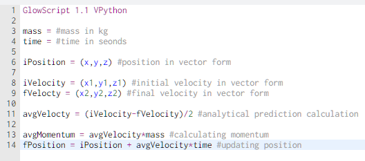

Not only does this code show how to use the analytical prediction method using python/GlowScript, it also shows how you can use that average velocity to calculate the momentum and update the position. These are the typical calculations associated with prediction methods.
Examples
Simple
A train is observed to be traveling at a speed of 24 m/s before it enters a city. While in the city, it is observed going 13 m/s. What is the average velocity of the train?
24 m/s + 13 m/s = 37 m/s
37/2 = 18.5
The average velocity of the train based on the analytical prediction method was 18.5 m/s. This average velocity can be used to determine the change in position as an application to this problem. This will be shown in the next example.
Middling
A car is traveling at a speed of (18, -2, 0) m/s. Later, the car is observed to be going (22, 6, 0) m/s. If the car started at the location (40, 170, 0) what is it's position after 30 seconds?
First, you have to find the average velocity:
(18, -2, 0) + (22, 6, 0) = (40, 4, 0)
(40, 4, 0) /2 = (20, 2, 0)
so the average velocity is (20, 2, 0) m/s
Second, calculate the change in position:
Change in position = average velocity x time
(20, 2, 0) * 30 = (600, 60, 0)
So the change in position is (600, 60, 0) m
Finally, update the position:
final position = initial position + change in position
(40, 170, 0) + (600, 60, 0) = (640, 230, 0)
The final position is (640, 230, 0) m
Difficult
A fan cart with m= 0.5Kg has the fan on and produces a net Force of <0.2,0,0>N, you give the cart a shove, and release the cart at position <0.5,0,0>m with initial velocity <0.3,0,0> m/s.
What is the momentum of the cart 0.6 seconds later?
Pf= <0.3,0,0>*.5 kgm/s + <0.2,0,0>*0.6 kgm/s = <0.27,0,0> kgm/s
What is its velocity at that time?
V = <0.27,0,0>kg m/0.5s kg = <0.54,0,0> m/s
Predict the position of the cart at that time.
XfCan be obtained in 4 different ways:
Xf= Xo+ Voxt + Fyt2/2m = 0.5 + 0.3*0.6+0.2*0.36/(2*.5) = 0.752m
Xf= Xo+ Vavgt, where Vavg= (Vox+Vfx)/2 = 0.5+(0.3+0. 54)/2)*0.6 = 0.752m
Xf= Xo+ Voxt + at2/2, where a= ΔV/Δt = 0.5+0.3*0.6+(.54-.3)*(0.6)2/( 2*.6) = 0.752m
Xf= Xo + (Vfx2 - Vo2)/2a = 0.5+(0.54*0.54-0.3*0.3)/(2*0.4) = 0.752m
Connectedness
1. How is this topic connected to something that you are interested in? Since this topic is based on such a fundamental mathematical principle, my interest in it lies in how wide spread this principle can be used not only in physics but in many other applications, fields, and scenarios. I wonder if this prediction is ever really used in the real world because in most times, force is not constant and the iterative method gives a more correct answer than the approximation. I do believe that this model is useful in ideal examples, but realistically, it must be hard.
2. How is it connected to your major? As stated in the previous connection, this basic principle has ties in just about every major with any connection to math including business, sciences, and engineering. Specifically, methods like this are often used to try and model basic relationships of properties in material science. My major is industrial engineering, so I believe this model can be applied to a lot of fields to calculate the efficiency and model a strategic way to eliminate waste.
3. Is there an interesting industrial application? In industry, methods like this, or methods very similar, are used every day to help process and analyze data in a very basic and quick way. If one is running out of time and does not have time to attempt an iterative motion or a program that will iteratively solve the problem, I believe this is useful to get a good approximation.
History
Historically, it is well known that basic algebra was discovered and implemented well before calculus, especially based on the fact that algebra was used as a basis to develop calculus. For this reason, it can be assumed that the analytical approach to physics problems related to velocity, or any other changing value, was used long before the iterative method. There is no information on who would have used this approach or when this approach was first used in a physics application.
See also
Vectors, Momentum Principle, Iterative Prediction, Forces, Velocity, Displacement
Further reading
There are several easily accessible resources with more information on analytical prediction methods and arithmetic means.
External links
References
http://www.platinumgmat.com/gmat_study_guide/statistics_mean (information) http://ncalculators.com/statistics/group-arithmetic-mean.htm (image) https://quizlet.com/24263897/mcat-physics-formulas-flash-cards/ (image) http://mathinsight.org/approximating_nonlinear_function_by_linear (image)