Electric Field
The Main Idea
In this page, the concept of an electric field produced by an electric point charge will be described qualitatively and quantitatively through models, examples, and a simulation. An electric field is a useful concept to describe how any charged particle would affect charge around it through the Coulomb force.
The electric field of a point charge is spherically symmetric, meaning it is the same at all points of equal radius from the source. Hence, it is useful to speak of the electric field at a certain radius (not at a certain [math]\displaystyle{ (x,y,z) }[/math] position), which will be done in the mathematical model.
Keep in mind, the electric field is a vector quantity. meaning it has a magnitude and direction. The SI units are N/C.
A Mathematical Model
The electric field vector [math]\displaystyle{ \bigl( \mathbf{E}_{s} \bigl) }[/math] of a point source charge [math]\displaystyle{ \bigl( Q_{s} \bigl) }[/math] gives the magnitude and direction of the electrostatic force vector [math]\displaystyle{ \bigl( \mathbf{F}_{s} \bigl) }[/math] exerted on a unit charge ([math]\displaystyle{ 1 }[/math] Coulomb) by [math]\displaystyle{ Q_{s} }[/math], as a function of position [math]\displaystyle{ \bigl( \mathbf{r} = (x,y,z) \bigl) }[/math]. More generally however, the electrostatic force vector exerted on any point charge [math]\displaystyle{ \bigl( q \bigl) }[/math] by a point source charge [math]\displaystyle{ \bigl( Q_{s} \bigl) }[/math] is related to the source charge's electric field vector by:
- [math]\displaystyle{ \mathbf{F}_{s} ( \mathbf{r} ) = |q| \mathbf{E}_{s} ( \mathbf{r} ) }[/math]
This definition requires an understanding of the electrostatic force (Coulomb's Law), and its mathematical description. If you are not familiar with this yet, read over the Electric Force page and come back.
Since the electric force is defined as:
- [math]\displaystyle{ \mathbf{F}( \mathbf{r} ) = \frac{1}{4\pi\epsilon_{o}}\frac{|q_{1} q_{2}|}{r^{2}} \hat{\mathbf{r}} }[/math], where
- [math]\displaystyle{ \epsilon_{o} }[/math] is the permittivity of free space with a value of [math]\displaystyle{ 8.854 \times 10^{-12} \frac{\text{C}^2}{\text{N} \cdot \text{m}^2} }[/math]
- [math]\displaystyle{ q_{1} }[/math] and [math]\displaystyle{ q_{2} }[/math] are point charges one and two, respectively
- [math]\displaystyle{ r }[/math] is the distance between the two point charges, which can also be written as [math]\displaystyle{ |\mathbf{r}| }[/math], the magnitude of the vector connecting the two charges' positions
- [math]\displaystyle{ \hat{\mathbf{r}} }[/math] is the unit vector pointing from charge one to charge two, or from charge two to charge one, depending on whether the force on charge two or charge one is wanted.
- [math]\displaystyle{ \mathbf{F}( \mathbf{r} ) = \frac{1}{4\pi\epsilon_{o}}\frac{|q_{1} q_{2}|}{r^{2}} \hat{\mathbf{r}} }[/math], where
The electric field of a source charge [math]\displaystyle{ Q_{s} }[/math] is:
- [math]\displaystyle{ \begin{align} \mathbf{E}_{s} ( \mathbf{r}) & = \frac{\mathbf{F}_{s} ( \mathbf{r} )}{|q|} \\ & = \frac{1}{4\pi\epsilon_{o}}\frac{|Q_{s}|}{r^{2}}\hat{\mathbf{r}} \end{align} }[/math]
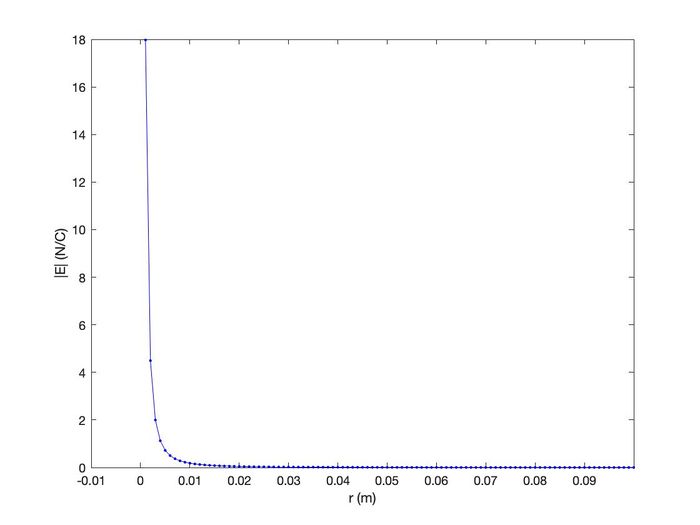
Radially, the magnitude of a charge's electric field looks something like this:
A point charge's electric field is also related to its electric potential. If you are unfamiliar with the idea of electric potential, then review these pages (Electric Field and Electric Potential and Electric Potential) and come back.
A charge's electric field and electric potential [math]\displaystyle{ V }[/math] are related by:
- [math]\displaystyle{ V_{ab} = -\int_{\mathbf{b}}^{\mathbf{a}} \mathbf{E} \cdot d\mathbf{L} }[/math], where
- [math]\displaystyle{ V_{ab} }[/math] is the potential difference between points [math]\displaystyle{ \mathbf{a} }[/math] and [math]\displaystyle{ \mathbf{b} }[/math]
- [math]\displaystyle{ \mathbf{E} }[/math] is the electric field
- [math]\displaystyle{ d\mathbf{L} }[/math] is an infinitesimal length in the direction of the path between [math]\displaystyle{ \mathbf{a} }[/math] and [math]\displaystyle{ \mathbf{b} }[/math]
- [math]\displaystyle{ V_{ab} = -\int_{\mathbf{b}}^{\mathbf{a}} \mathbf{E} \cdot d\mathbf{L} }[/math], where
This relation is less useful for us unless we use a straight line approximation, such that:
- [math]\displaystyle{ \begin{align} V_{ab} & = -\mathbf{E} \cdot \Delta \mathbf{L} \\ & = - \bigl( E_{x}, E_{y}, E_{z} \bigl) \cdot \bigl( \Delta L_{x}, \Delta L_{y}, \Delta L_{z} \bigl) \\ & = - \bigl( E_{x}\Delta L_{x} + E_{y}\Delta L_{y} + E_{z}\Delta L_{z} \bigl) \\ \end{align} }[/math]
This leads to:
- [math]\displaystyle{ \mathbf{E} (x,y,z) = - \biggl( \frac{\Delta V_{x}}{\Delta L_{x}}, \frac{\Delta V_{y}}{\Delta L_{y}}, \frac{\Delta V_{z}}{\Delta L_{z}} \biggl) }[/math]
By convention, the electric field due to a positive point charge always points away from itself, and the electric field of a negative point charge always points towards itself as shown below:

Different charges will attract each other, and like charges will repel each other, as shown below:

Lastly, the principle of superposition is directly applicable to finding the electric field due to multiple point source charges, using the a vector sum:
- [math]\displaystyle{
\begin{align}
\mathbf{E}_{sum} (\mathbf{r}) & = \mathbf{E}_{1} + \mathbf{E}_{2} + \mathbf{E}_{3} + \cdots + \mathbf{E}_{N} \\
& = \sum_{1}^{N} \mathbf{E}_{n} \\
& = \sum_{1}^{N} \frac{1}{4 \pi \epsilon_{o}} \frac{|Q_{s_{n}}|}{r_{n}^{2}} \hat{\mathbf{r}}_n
\end{align}
}[/math]
- When using this, be careful to add the positive charges and negatives charges separately, since their fields point in opposite directions. A negative will need to be applied to the negative electric field sum.
- [math]\displaystyle{
\begin{align}
\mathbf{E}_{sum} (\mathbf{r}) & = \mathbf{E}_{1} + \mathbf{E}_{2} + \mathbf{E}_{3} + \cdots + \mathbf{E}_{N} \\
& = \sum_{1}^{N} \mathbf{E}_{n} \\
& = \sum_{1}^{N} \frac{1}{4 \pi \epsilon_{o}} \frac{|Q_{s_{n}}|}{r_{n}^{2}} \hat{\mathbf{r}}_n
\end{align}
}[/math]
- Critical Formulas:
- [math]\displaystyle{ \mathbf{E} ( \mathbf{r}) = \frac{\mathbf{F} ( \mathbf{r} )}{|q|} }[/math]
- [math]\displaystyle{ \mathbf{E} ( \mathbf{r}) = \frac{1}{4\pi\epsilon_{o}}\frac{|Q|}{r^{2}}\hat{\mathbf{r}} }[/math]
- [math]\displaystyle{ \mathbf{E} (x,y,z) = - \biggl( \frac{\Delta V_{x}}{\Delta L_{x}}, \frac{\Delta V_{y}}{\Delta L_{y}}, \frac{\Delta V_{z}}{\Delta L_{z}} \biggl) }[/math]
- [math]\displaystyle{ \mathbf{E}_{sum} (\mathbf{r}) = \sum_{1}^{N} \frac{1}{4 \pi \epsilon_{o}} \frac{|Q_{s_{n}}|}{r_{n}^{2}} \hat{\mathbf{r}}_n }[/math]
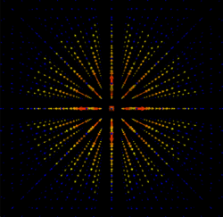
A Computational Model
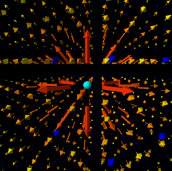
   ###--Create Electric Field Lines of a Positive Charge at the Origin--###
   #==============================================================#
   #---Import statements for VPython---#
   from __future__ import division
   from visual import *
   #---Import function used to find combinations---#
   from itertools import combinations
   #==============================================================#
   #---Create scene---#
   scene.center = vector(0,0,0)  #-Position of source charge-#
   scene.height = 800  #-Set height of frame of scene-#
   scene.width = 800  #-Set width of frame of scene-#
   scene.range = 4  #-Set range of scene-#
   scene.userzoom = 1  #-Allow user to zoom in/out: CTRL & move in/out on trackpad-#
   scene.userspin = 1  #-Allow user to rotate camera angle: SHIFT & OPTION & move around on track pad-#
   #==============================================================#
   #---Specify point charge attributes---#
   sourceCharge = 3*10**(-11)  #-Coulombs of charge-#
   sourcePos = vector(0,0,0) #-Position of source charge-#
   ###--Modeling source point charge as a sphere with radius 0.1 meters--###
   sourceObj = sphere(pos = sourcePos, radius = 0.1, color = color.cyan)
   #==============================================================#
   #---Set range (0 to 3) and possible inputs for the coordinates (0.5 step)---#
   ###--Many of the same number included to allow for combinations such as (1,1,1).
       #The itertools.combinations function will only use each element of the...
       #list once, starting from the beginning.
       #Repeating each coordinate many times with intermixing, grants...
       #all combinations of points, with repeats however.
       #Later, a for loop will be used to eliminate repeats.
       #This can be optimized later if need be.---------------###
   posXYZ = [0, -0.5, 1, -1.5, 2, -2.5, 3,
             0, 0.5, -1, 1.5, -2, 2.5, -3,
             0, -0.5, 1, -1.5, 2, -2.5, 3,
             0, 0.5, -1, 1.5, -2, 2.5, -3,
             0, -0.5, 1, -1.5, 2, -2.5, 3,
             0, 0.5, -1, 1.5, -2, 2.5, -3,
             0, -0.5, 1, -1.5, 2, -2.5, 3,
             0, 0.5, -1, 1.5, -2, 2.5, -3,
             0, -0.5, 1, -1.5, 2, -2.5, 3,
             0, 0.5, -1, 1.5, -2, 2.5, -3,
             0, -0.5, 1, -1.5, 2, -2.5, 3,
             0, 0.5, -1, 1.5, -2, 2.5, -3]
   #==============================================================#
   #---Create combinations of points (x,y,z) for later use---#
       ###--prelimPoints will be a list of tuples of tuples--##
           #ie: [((,,),(,,),(,,),(,,)) , ((,,),(,,)) ,..., ((,,),(,,))]
   prelimPoints = [tuple(combinations(posXYZ, 3))]
   ###--Pull the points out of the grouping tuples and add them to a...
       #new list alphaPoints------------------------###
   alphaPoints = []
   for groupingTuple in prelimPoints:
       for XYZ in groupingTuple:
           if XYZ not in alphaPoints:  #-Check for repeat (x,y,z)-#
               alphaPoints.append(XYZ)
           ##--The negative of this tuple may not be in the combinations:
               #check to see-------------##
           first = -XYZ[0]
           second = -XYZ[1]
           third = -XYZ[2]
           negXYZ = (first, second, third)
           if negXYZ not in alphaPoints:
               alphaPoints.append(negXYZ)
           ##--Swap x and z coordinates for futher combination checking--##
           first = XYZ[2]
           second = XYZ[1]
           third = XYZ[0]
           reverseXYZ = (first, second, third)
           if reverseXYZ not in alphaPoints:
               alphaPoints.append(reverseXYZ)
           ##--The negative of the x and z coordinate swap may not be in...
               #the combinations: check to see---------##
           first = -XYZ[2]
           second = -XYZ[1]
           third = -XYZ[0]
           reverseXYZneg = (first, second, third)
           if reverseXYZneg not in alphaPoints:
               alphaPoints.append(reverseXYZneg)
           ##--Make x [3], y [0], and z [1] to check for more combinations--##
           first = XYZ[1]
           second = XYZ[2]
           third = XYZ[0]
           shiftedXYZ = (first, second, third)
           if shiftedXYZ not in alphaPoints:
               alphaPoints.append(shiftedXYZ)
           ##--The negative of the shifted XYZ may not be in the combinations:
               #check to see---------------##
           first = -XYZ[1]
           second = -XYZ[2]
           third = -XYZ[0]
           shiftedXYZneg = (first, second, third)
           if shiftedXYZneg not in alphaPoints:
               alphaPoints.append(shiftedXYZneg)
   ###--------This should be enough recombining---------###
   #================================================================#
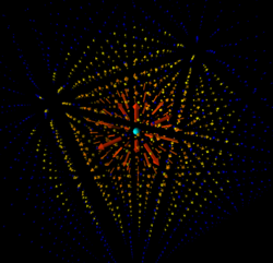
   #---Create a new list of tuples that contain the points, magnitude,...
       #and direction (betaPoints)-----------#
           #ie: [((x,y,z), mag((x,y,z)), norm((x,y,z))),...]
   betaPoints = []
   for XYZ in alphaPoints:
       Mag = mag(XYZ)
       Dir = norm(XYZ)
       betaPoints.append((XYZ, Mag, Dir))
   #================================================================#
   #---Sort the tuples based on their magnitudes from least to greatest...
      #using sorted().
           #key = lamda x: x[1] tells the sorted function to sort the tuples...
               #based on their second component...their magnitudes--------#
   charliePoints = sorted(betaPoints, key = lambda x: x[1])
   #================================================================#
   #---Calculate parts of electric field equation:
       #E = 1/(4*pi*epsilon0) * Q/(magnitude)**2
   epsilonO = 8.854*(10**(-12)) #-N*(m/C)**2-#
   k = 1/(4*pi*(epsilonO)) #-N*(m/C)**2-#
   chargeContri = k*sourceCharge #-N*(m**2/C)-#
   #================================================================#
   #---Loop through points and find mag of electric field:
       #add it to a new list with the existing tuple info-------#
   deltaPoints = []
   for XYZ in charliePoints:
       try:  ###-Avoid divide by 0 error in (x,y,z) = (0,0,0)-###
           magEfield = chargeContri*(1/(XYZ[1])**2)
       except:
           magEfield = 0
       tupEfield = (XYZ[0], XYZ[1], XYZ[2], magEfield)
       deltaPoints.append(tupEfield)
   #================================================================#
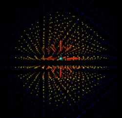
   #---Loop through points and create an arrow at that point proportional in...
       #length to the magnitude of the electric field there.
       #Also, the arrow points in the direction of the electric field there.
       #Color coding is based on 0.25 meter increments:
           #stronger field = redder; weaker field = blue
   for XYZ in deltaPoints:
       if XYZ[1] <= 0.25:
           lengthP = XYZ[3]*0.5
           arroW = arrow(pos=vector(XYZ[0]), axis=XYZ[2],
                         color = vector(1.000, 0.000, 0.000),
                         length = lengthP,
                         headwidth = lengthP*0.2,
                         headlength = lengthP*0.25)
       elif XYZ[1] <= 0.5:
           lengthP = XYZ[3]*0.7
           arroW = arrow(pos=vector(XYZ[0]), axis=XYZ[2],
                         color = vector(1.000, 0.200, 0.000),
                         length = lengthP,
                         headwidth = lengthP*0.2,
                         headlength = lengthP*0.25)
       elif XYZ[1] <= 1:
           lengthP = XYZ[3]*0.9
           arroW = arrow(pos=vector(XYZ[0]), axis=XYZ[2],
                         color = vector(1.000, 0.300, 0.000),
                         length = lengthP,
                         headwidth = lengthP*0.2,
                         headlength = lengthP*0.25)
       elif XYZ[1] <= 1.25:
           lengthP = XYZ[3]*1.1
           arroW = arrow(pos=vector(XYZ[0]), axis=XYZ[2],
                         color = vector(1.000, 0.400, 0.000),
                         length = lengthP,
                         headwidth = lengthP*0.2,
                         headlength = lengthP*0.25)
       elif XYZ[1] <= 1.5:
           lengthP = XYZ[3]*1.3
           arroW = arrow(pos=vector(XYZ[0]), axis=XYZ[2],
                         color = vector(1.000, 0.500, 0.000),
                         length = lengthP,
                         headwidth = lengthP*1,
                         headlength = lengthP*1)
       elif XYZ[1] <= 1.75:
           lengthP = XYZ[3]*1.5
           arroW = arrow(pos=vector(XYZ[0]), axis=XYZ[2],
                         color = vector(1.000, 0.600, 0.000),
                         length = lengthP,
                         headwidth = lengthP*1,
                         headlength = lengthP*1)
       elif XYZ[1] <= 2:
           lengthP = XYZ[3]*1.7
           arroW = arrow(pos=vector(XYZ[0]), axis=XYZ[2],
                         color = vector(1.000, 0.700, 0.000),
                         length = lengthP,
                         headwidth = lengthP*1,
                         headlength = lengthP*1)
       elif XYZ[1] <= 2.25:
           lengthP = XYZ[3]*1.9
           arroW = arrow(pos=vector(XYZ[0]), axis=XYZ[2],
                         color = vector(1.000, 0.800, 0.000),
                         length = lengthP,
                         headwidth = lengthP*1,
                         headlength = lengthP*1)
       elif XYZ[1] <= 2.5:
           lengthP = XYZ[3]*2.1
           arroW = arrow(pos=vector(XYZ[0]), axis=XYZ[2],
                         color = vector(1.000, 0.900, 0.000),
                         length = lengthP,
                         headwidth = lengthP*1,
                         headlength = lengthP*1)
       elif XYZ[1] <= 2.75:
           lengthP = XYZ[3]*2.3
           arroW = arrow(pos=vector(XYZ[0]), axis=XYZ[2],
                         color = vector(1.000, 1.000, 0.000),
                         length = lengthP,
                         headwidth = lengthP*1,
                         headlength = lengthP*1)
       else:
           lengthP = XYZ[3]*2.5
           arroW = arrow(pos=vector(XYZ[0]), axis=XYZ[2],
                         color = color.blue,
                         length = lengthP,
                         headwidth = lengthP*1,
                         headlength = lengthP*1)
- Also, at this link Charges and Fields is a PhET simulation of electric fields. Play with it if you like.
Examples
Simple
- Question:
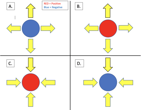
- In the following figure, the red circles represent positive point charges, and the blue circles represent negative point charges. If the yellow arrows are meant to represent the point charge's electric field lines, which field(s) and charge(s) are correctly matched? (Only take into account direction)
- Solution:
- Since electric field lines always point away from a positive point charge, Option (C.) cannot be correct. Likewise, electric field lines always point towards a negative charge. Therefore, Option (A.) is also incorrect.
- Option (B.) shows a positive charge with an electric field pointing radially outwards. This is correct. Option (D.) shows a negative charge with an electric field pointing radially inwards. This is also correct.
- Answer: Options (B.) & (D.)
Middling
Difficult
Connectedness
History
See also
Further reading
External links
References
The Main Idea
The main idea of this page is to develop an understanding of electric fields and the types of particles that produce electric fields.
History
Electric fields are created by electric charges. The original discovery of the electric charge is not explicitly known, but in 1675 the esteemed chemist Robert Boyle, known for Boyle's Law, discovered the attraction and repulsion of certain particles in a vacuum. Almost 100 years later in the 18th century the American Benjamin Franklin first coined the phrases positive and negative (later developed into proton and electron) for these particles with attractive and repulsive properties. Finally, in the 19th century Michael Faraday utilized his electrolysis process to discover the discrete nature of electric charge.
Electric Field
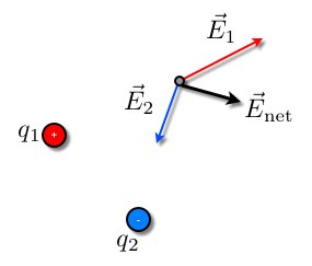
Electric Field is a field created by an electric charge. It is measured in units of newtons per coulomb (N/C), the proper units of which are (kg*(m/s^2)), and has a direction, making it a vector quantity. Electric fields can also be in the units of volts per meter (V/m). The electric field created by a charge exists at all points in space and exerts a force on other charged objects. The field can be drawn as an arrow with tail at the observation location pointing in the direction of the field. The Electric field obeys superposition, so the net Electric field at a point in space can be determined by summing all the individual fields present at that location.
The electric field of a positive particle points away from the particle, while the electric field of a negative particle points toward the particle, as seen right here:

When two oppositely charged particles are placed next to each other, their electric field moves from the positive to the negative. Two similarly charged particles will have fields that are repelled by each other. This is shown below:
The two oppositely charged particles, when in very close proximity, will act together in the form of a dipole.
Mathematical Concept of a Field
In mathematics, a field is a value that exists at all points in space. The magnitude of an electric field is a scalar. The field itself is represented as a vector: <x,y,z>. Other examples of fields are gravitational fields and magnetic fields.
You can calculate electric field in a few ways. You can calculate the electric field vector and magnitude by using the following equations:
[math]\displaystyle{ E = \frac{F}{q} }[/math], where F is the force and q is the charge of the particle. This formula is very helpful to think about to understand the relation between force and electric field.
[math]\displaystyle{ E = \frac{kQ}{r^2} }[/math], where k is Coulomb's constant, or 9x10^9, Q is the charge of the particle, and r is the distance between both particles.
The magnitude of an electric field can be also be calculated by using the potential difference, Δϕ, between two plates and the distance, d, between them.
- [math]\displaystyle{ E = -\frac{\Delta\phi}{d} }[/math]
Electric Field and Force
The force due to an external electric field on a charged particle is given by the equation [math]\displaystyle{ \vec{F} = q\vec{E} }[/math] where q is the charge of the observed particle and E is the electric field. The field created by a charged particle exerts no force on itself. This is to say that the force on a given particle is defined as the charge on that particle multiplied the combined electric fields of the external environment. Since force is measured in Newtons (N) and charge in Coulombs (C), Electric field is measured in Newtons per Coulomb (N/C) as mentioned earlier. Furthermore, the magnitude of an electric field is not dependent on the sign of q (i.e. whether the charge is positive or negative.) The sign only helps determine the direction that the electric field points.
To calculate the electric force on a particle, first you must calculate the electric fields affecting the particle. Applying superposition, you add all electric fields to find the net field. Once you have this, you multiply the electric field by the charge of the particle, and this gives you the force exerted on the particle. Like charges repel each other and opposite charges attract each other.
Electric Field and Superposition
The electric field contributed by a charged particle is unaffected by the electric field contributed by other charged particles. To that end, the principle of superposition, as mentioned earlier, states that the net electric field at a location is determined by the sum of all individual electric fields on charged particles. The principle of superposition is very useful to determine the force on a given charged particle. By being able to define electric field as a vector and simply adding up the various components of individual electric fields, the force on a particle is easily calculated using [math]\displaystyle{ \vec{F} = q\vec{E} }[/math]
The two must common methods of combining vectors in the principle of superposition are the tail to tail method (number 1 in the image below) and head to tail (number 2 in the image below).
Electric Field and Electric Potential
Another way to define electric field is using the electric potential over a certain distance to determine field. Electric potential is referred to as electric field potential or electrostatic potential. In this case, Electric field is shown in units volts (V) per meter (m) (V/m). Again, electric field is calculated with potential difference with the equation: [math]\displaystyle{ E = -\frac{\Delta\phi}{d} }[/math]
Examples
Simple
Select all of the arrows that accurately show the electric field produced by the charge shown. (only direction not magnitude)
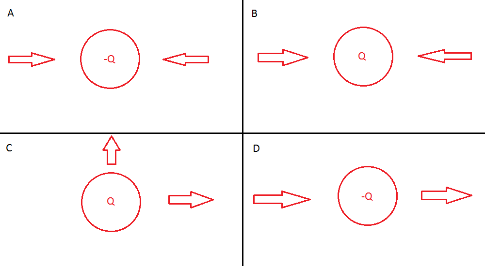 We know that the electric field from a single point charge will always point outwards if it is positive and always inwards if it is negative. This means that A and C are both correct. It is also important to remember that opposites will attract. In this case a negative and positive charge will attract to one another in any orientation. It is also important to remember that oppositely charged particles will repel each other, so any negative-negative or positive-positive interaction will result in a repelling force.
Middling
What is the magnitude and direction of the electric field at the origin (assume Q = 1 coulomb)?
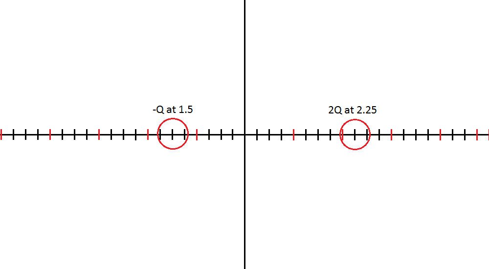
There is a positive charge on the right with an electric field pointing to the left at the origin. The negative charge on the left also has an electric field pointing to the left at the origin so we will add the two electric fields as they point along the negative x axis. [math]\displaystyle{ \frac{k}{1.5^2}+\frac{k*2}{2.25^2} = 0.75*10^{10} }[/math]. This is a similar mathematical representation to the image in electric field and superposition section of this page. The force of the positive and negative charges are both acting on the specific reference point and have a total Enet value that is the combination of the two opposite forces. The Enet in this scenario is the 0.75*10^{10} </math> value that was calculated in the +x direction.
Difficult
What is the magnitude of the electric field experienced by the positive particle at the top of the triangle?
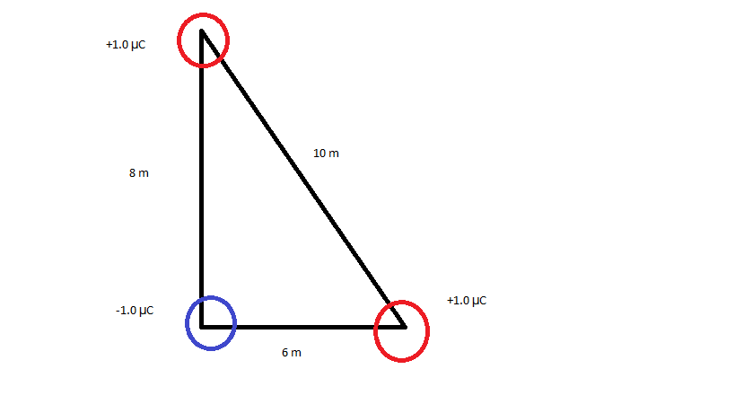
The first step is to find the angle measure of the angle that is opposite of the 8 meter side of the triangle. To do this you must use inverse cosine to find the angle measure. Then we have to find the electric field caused by the other two particles at the point we are analyzing. We need to split the electric field at the point to its x- and y- components. The magnitude of the electric field caused by the positive particle is the following: E= ((9×〖10〗^9)(1×〖10〗^(-6)))/100=90. The negative particle has the following magnitude: E= ((9×〖10〗^9)(1×〖10〗^(-6)))/64=140.63.No we look at the x- component of the electric field. The negative particle does not create a electric field in the x-direction at the observation location. The positive particle has an electric field of cos(53.13) times the magnitude of the electric field. The electric field in the y-direction is the magnitude of the negative particle and sin(53.13) times the magnitude of the positive particle. The vector for the electric field at the point is as follows: (-54,-68.63). Now we have to find the magnitude of this vector to find the magnitude of the electric field at the observation location. The magnitude is 87.33 N/C.
VPython
An arrow can be coded to represent the direction of the electric field at a point in VPython by using the formula for the electric field at a point.
![]()
The first step is to define any constants needed. Oofpez (one over four pi epsilon naught) should be defined as 9e9. The charge of the particle creating an electric field should also be defined.
The second step is to create the particle, which is usually either a proton or an electron.
The third step is to create an observation location, which can be titled obslocation.
The fourth step should be to calculate the electric field. Start by defining r, the distance from the observation location to the particle. Next, determine the magnitude of r and r hat. Then, plug all values in to determine the electric field at the observation location.
The fifth step is to create an arrow to represent the direction of the electric field.
Example
Create an arrow at location <5e-10,0,0> to represent the direction of the electric field generated from a proton located at <2e-10,0,0>.
-CONSTANTS-
oofpez = 9e9
q = 1.6e-19
-OBJECTS-
proton = sphere(pos=vec(2e-10,0,0), radius=1e-11, color=color.red)
-INITIAL VALUES-
obslocation = vec(5e-10,0,0)
-CALCULATIONS-
r = obslocation-proton.pos
rmag = sqrt((r.x)**2 + (r.y)**2 + (r.z)**2)
rhat = (r)/(rmag)
Enet = ((oofpez)*(q)/(rmag**2))*(rhat)
-OBJECTS-
Efield = arrow(pos=obslocation, axis=Enet, color=color.orange)
Uses of Electric Fields
Electric Motors
Electric motors convert electrical energy into mechanical energy through electric fields. Whenever electric motors are turned on, electric fields are generated. This is because in order to turn an electric motor, an electric field must first be generated, which then generates a magnetic field, thus making the motor spin. Electric motors are used in cars, elevators, fans, refrigerators, and many more applications.
Computers
In order for computers to run, an electric fan motor must run. As previously mentioned, for electric motors to run, an electric field must be generated. Therefore, electric fields are what allow for us to use modern day computers.
Paintings
Electric fields are also used in some paintings. The electric field generates charges on the surface of the material being painted on, and an opposite charge is generated on the paint. Paint that touches the material sticks, and excess paint falls off to go back into the system.
Cancer Treatment
Recently, weak electric fields have been used to kill cancer cells. This treatment works best for brain and breast cancers, and it has no effect on normal cells. In lab and animal tests, this treatment killed cancer cells of every type tested; however, this is still a developing treatment.
Connectedness
The ability to understand electric fields helps set the basis for the introduction of Electric Force (as we discussed [math]\displaystyle{ \vec{F} = q\vec{E} }[/math] ). The introduction of electric force will attach the specific charge of the particles with the electric field that they produce, resulting in the electric force. Electric force will lay the ground work for understanding the force that particles have in different systems and environments, and eventually lead to the introduction of Magnetic Force.
See also
The understanding of electric fields is a doorway into all the various fields only some of which will be covered in physics 2212. The fundamental understanding of electric fields will prove to be very important further along when magnetic fields are introduced as they share many qualities. The understanding of electric and magnetic fields will be used throughout the semester to learn about various electromagnetic concepts, and ultimately a understanding and application of Maxwell's Equations. Please see related topics:
External links
A youtube playlist that does a great job going step by step and reviewing topics
Further review on electric field lines.
References
This section contains the the references you used while writing this page

