Electric Field
CLAIMED BY PRANEETHA VISHNUBHOTLA - FALL 2025
The Main Idea
The electric field describes how an electrically charged particle or group of particles (source charge) would affect other electrically charged objects (test charge) placed in the field. The familiar electric force may be viewed as a consequence of the test charge's interaction with the field. Every position vector [math]\displaystyle{ \vec{r} = \lt x, y, z\gt }[/math] (also works for other coordinate systems) can be associated with an electric field vector [math]\displaystyle{ \vec{E}(\vec{r}) }[/math]. Electric fields follow the superposition principle. If there are multiple source charges, the net field at a given point equals the sum of the individual fields produced by each source charge. Note the electric field is a vector, meaning it has a direction [math]\displaystyle{ \hat{E} }[/math] and a magnitude [math]\displaystyle{ E }[/math]. It is measured in N/C (Newtons per Coulomb) or V/m (Volts per meter), depending on which representation is more meaningful in context.
A Mathematical Model
The electric field can be defined from the electric force on a test charge: [math]\displaystyle{ \vec{F} = q\vec{E} \quad \Rightarrow \quad \vec{E} = \frac{\vec{F}}{q}. }[/math]
For a single point charge [math]\displaystyle{ Q }[/math] at distance [math]\displaystyle{ r }[/math], the electric field is [math]\displaystyle{ \vec{E}(\vec r) = \frac{1}{4\pi\epsilon_{0}} \frac{Q}{r^{2}} \hat{r}, }[/math] where [math]\displaystyle{ \hat r }[/math] is the unit vector pointing from the source charge to the observation point.
If there are multiple point charges, the net field is found by superposition: [math]\displaystyle{ \vec{E}_{\text{net}}(\vec r) = \sum_{i=1}^{N} \vec{E}_{i}(\vec r). }[/math] The above is basically saying you add up each E-field vector for the specific point in space from each external E-field.
The electric field is also related to the electric potential [math]\displaystyle{ V }[/math] by [math]\displaystyle{ \vec{E} = -\nabla V = \left\langle -\frac{\partial V}{\partial x},\, -\frac{\partial V}{\partial y},\, -\frac{\partial V}{\partial z} \right\rangle. }[/math]
This is using Calculus. You can also take the approach without using Calculus:
Electric field points in the direction of the greatest decrease in electric potential, and its magnitude tells how quickly the potential is dropping at a point in space. Protons move from high potential to low potential, thus following: [math]\displaystyle{ U = qV }[/math]
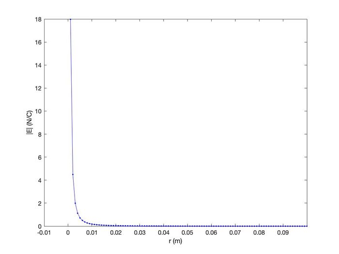
Note the inverse-square relationship between the magnitude of the field [math]\displaystyle{ E }[/math] and the distance [math]\displaystyle{ r }[/math]. Also note that [math]\displaystyle{ r }[/math] cannot equal 0, so there is no self-interaction between a point charge and itself. The asymptote at [math]\displaystyle{ r = 0 }[/math] m and the magnitude of the electric field [math]\displaystyle{ E }[/math] decaying by a factor of [math]\displaystyle{ r^{2} }[/math] can be seen below:
Using Superposition
The [math]\displaystyle{ \vec{E} = \frac{1}{4\pi\epsilon_{0}}\frac{Q}{r^{2}}\hat{r}_{ } }[/math] equation is valid for a single point charge. By the superposition principle, we can use this equation to find the electric field of more complicated structures like dipoles, quadrupoles, lines, spheres, shells, planes, etc. The sum can be expressed as follows: [math]\displaystyle{ \vec{E}_{net} = \sum_{i=1}^{N}\vec{E}_{i} = \vec{E}_{1} + \vec{E}_{2} + \cdots + \vec{E}_{N} }[/math]
- [math]\displaystyle{ \vec{E}_{i} }[/math] refers to the field produced by one point charge
- [math]\displaystyle{ N }[/math] refers to the total number of point charges
Using Electric Potential
This is a little bit of additional information on Electric Potential:
The electric field is also related to the electric potential [math]\displaystyle{ V }[/math] (not discussed at the start of the course): [math]\displaystyle{ \Delta V = V(\vec{r_{f}}) - V(\vec{r_{i}}) = -\int_{\vec{r_{i}}}^{\vec{r_{f}}} \vec{E}(\vec{r}) \cdot \vec{dl} = - \int_{x_{i}}^{x_{f}} E_{x}dx - \int_{y_{i}}^{y_{f}} E_{y}dy - \int_{z_{i}}^{z_{f}} E_{z}dz \Rightarrow \vec{E} = - \nabla V = \lt - \frac{\partial V}{\partial x}, - \frac{\partial V}{\partial y}, - \frac{\partial V}{\partial z}\gt }[/math]
- [math]\displaystyle{ \vec{r_{f}} }[/math] and [math]\displaystyle{ \vec{r_{i}} }[/math] represent the final and initial positions
- [math]\displaystyle{ \vec{dl} }[/math] represents an infinitesimal length along any path
- [math]\displaystyle{ \nabla V }[/math] represents the gradient of the voltage
Coulomb and Non-Coulomb Electric Fields
Coulomb Electric Fields: Coulomb Electric Fields are electric fields that come from charges that aren't moving or changing. For example, this includes: 1. Electric fields around a point charge 2. Between plates of a charged capacitor 3. In the vicinity of a charged sphere or rod
These have a conservative behavior, and thus Coulomb's law can be used to find the electric field. [math]\displaystyle{ \vec{E} = \frac{1}{4\pi\epsilon_{0}} \frac{Q}{r^{2}} \hat{r} }[/math]
Non-Coulomb Electric Fields: These fields are not produced by charges but are produced by changing electric fields. You can learn more about this by going to the Faraday's Law Portion of this Wiki. However, a basic overview of Faraday's Law is that a changing magnetic field through a coil of wire induces a current, which will create a magnetic field opposing/following the motion of the current, according to the right-hand rule, according to how the magnetic flux is changing.
If the flux is increasing, the induced field and current will be the opposite direction to decrease the change in /vec{B}.
If the flux is decreasing, the induced field and current will be the same direction to increase the change in /vec{B}.
This can be seen in Faraday's Law: [math]\displaystyle{ \oint \vec{E} \cdot d\vec{\ell} = -\,\frac{d\Phi_{B}}{dt} }[/math] [math]\displaystyle{ \Phi_{B} = \int \vec{B} \cdot d\vec{A} }[/math]
A Computational Model
When visually drawing the electric field, the arrows point away from the positive charge and toward the negative charge. A stronger field strength can be represented by longer arrows or more densely packed arrows.
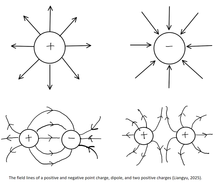
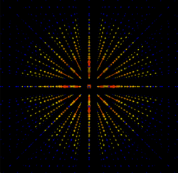
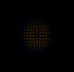
The following code can be used to visualize the electric field produced by a positive point charge. The interactive viewer may be found here: New field simulation code. Note that this code was not used to generate the exact images on this page. However, it is functionally identical and produces the same image; follow the link to find out for yourself. For reference, the old code may be found at the bottom of the page or this link: Old field simulation code.
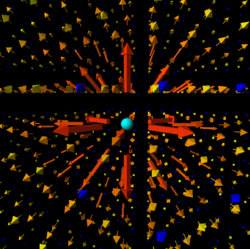
Web VPython 3.2
#Praneetha Vishnubhotla -- Fall 2025
scene.caption = """Right button drag or Ctrl-drag to rotate "camera" to view scene."""
scene.center = vector(0, 0, 0)
scene.height = 800
scene.width  = 800
scene.range  = 4

# Source charge at the origin
sourcePos = vector(0, 0, 0)
sourceObj = sphere(pos=sourcePos, radius=0.1, color=color.cyan)

# -------------------------------------------------
# CONSTANTS
# -------------------------------------------------
epsilon0 = 8.854e-12
k        = 1 / (4 * pi * epsilon0)
Q        = 3e-11                 # Coulombs
base     = k * Q                 # overall scale for |E|
globalScale = 1

maxR = 3
step = 0.5

for x in arange(-maxR, maxR + step, step):
    for y in arange(-maxR, maxR + step, step):
        for z in arange(-maxR, maxR + step, step):

            rvec = vector(x, y, z)
            rmag = mag(rvec)

            # Skip the origin so we don’t divide by zero
            if rmag == 0:
                continue

            rhat = norm(rvec)

            # |E| ~ kQ / r^2 (we only care about relative sizes)
            Emag = base / (rmag ** 2)

            # --------------------------------------------
            # Matching color of old code
            # --------------------------------------------
            if rmag <= 0.25:
                lengthP = Emag * 0.5
                acol    = vector(1.0, 0.0, 0.0)
            elif rmag <= 0.5:
                lengthP = Emag * 0.7
                acol    = vector(1.0, 0.2, 0.0)
            elif rmag <= 1.0:
                lengthP = Emag * 0.9
                acol    = vector(1.0, 0.3, 0.0)
            elif rmag <= 1.25:
                lengthP = Emag * 1.1
                acol    = vector(1.0, 0.4, 0.0)
            elif rmag <= 1.5:
                lengthP = Emag * 1.3
                acol    = vector(1.0, 0.5, 0.0)
            elif rmag <= 1.75:
                lengthP = Emag * 1.5
                acol    = vector(1.0, 0.6, 0.0)
            elif rmag <= 2.0:
                lengthP = Emag * 1.7
                acol    = vector(1.0, 0.7, 0.0)
            elif rmag <= 2.25:
                lengthP = Emag * 1.9
                acol    = vector(1.0, 0.8, 0.0)
            elif rmag <= 2.5:
                lengthP = Emag * 2.1
                acol    = vector(1.0, 0.9, 0.0)
            elif rmag <= 2.75:
                lengthP = Emag * 2.3
                acol    = vector(1.0, 1.0, 0.0)
            else:
                lengthP = Emag * 2.5
                acol    = color.blue

            # --------------------------------------------
            # E field arrows
            # --------------------------------------------
            axisVec = rhat * lengthP * globalScale

            arrow(pos=rvec,
                  axis=axisVec,
                  color=acol,
                  headlength=mag(axisVec) * 0.25,
                  headwidth =mag(axisVec) * 0.2)
This is the link to the GLowScript if you'd like to look at the image simulations: https://www.glowscript.org/#/user/pvishnubhotla6/folder/public/program/WikiTextbook
- This link Charges and Fields provides a PhET simulation of Electric Fields. Play with it!
- Or if you prefer something with more action, explore this Hockey Game to gain a deeper visual understanding of electric fields and their effects on charges
Examples
Simple
- Question:
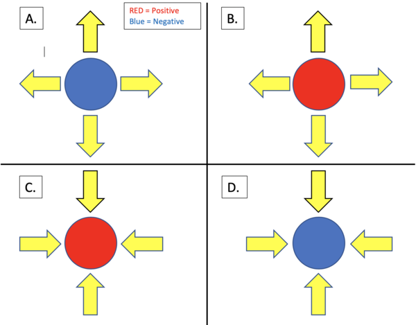
- In the following figure, the red circles represent positive point charges, and the blue circles represent negative point charges. If the yellow arrows are meant to represent the Electric Field due to each point charge, which field(s) and charge(s) are correctly matched? (Only take into account direction)
- Solution:
- Since Electric Field lines always point away from a positive point charge, Option (C.) cannot be correct. Likewise, Electric Field lines always point towards a negative charge. Therefore, Option (A.) is also incorrect.
- Option (B.) shows a positive charge with an Electric Field pointing radially outwards. This is correct. Option (D.) shows a negative charge with an Electric Field pointing radially inwards. This is also correct.
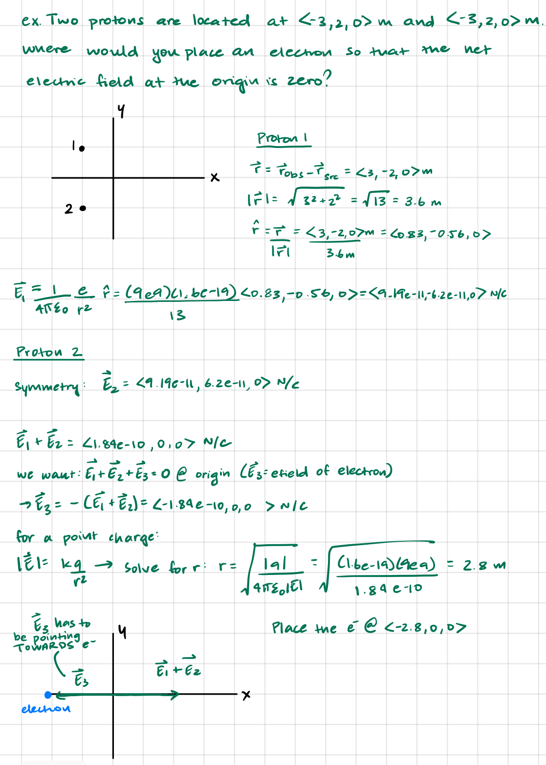
- More simple examples from class notes
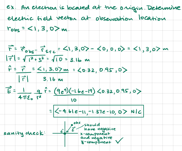
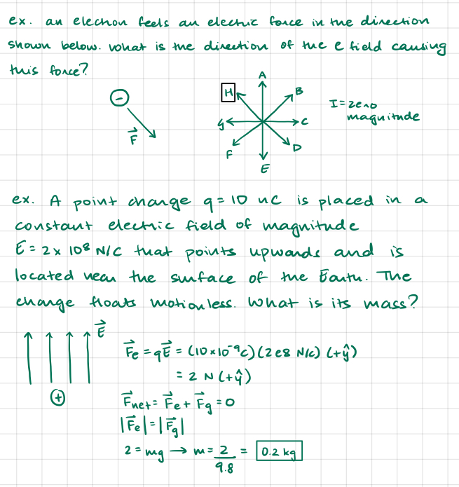
Middling
- Question:
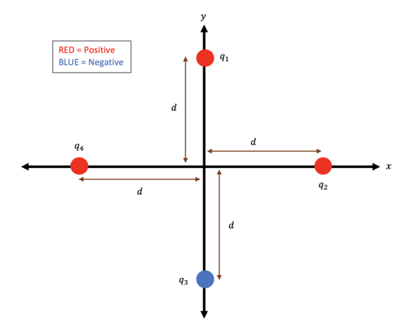
- Four point charges [math]\displaystyle{ \big(q_{1}, q_{2}, q_{3}, \text{and} \ q_{4} \big) }[/math], are each located at a distance [math]\displaystyle{ d }[/math] along either the [math]\displaystyle{ x }[/math] or [math]\displaystyle{ y }[/math] axes, as shown in the figure below. If [math]\displaystyle{ \ |q_{3}| = |q_{1}| \ \text{and} \ |q_{4}| = |q_{2}| }[/math] what does the Electric Field at the origin reduce to?
- Solution:
- A.) We can start by observing the geometry of the problem. We want the net field at the origin, and the distance between the origin and each point charge is identical. [math]\displaystyle{ r_{1} = r_{2} = r_{3} = r_{4} = d }[/math] We also need to find the unit vector [math]\displaystyle{ \hat{r} }[/math] that points from each point charge to the origin. [math]\displaystyle{ \hat{r_{1}} = -\hat{y}, \hat{r_{2}} = -\hat{x}, \hat{r_{3}} = \hat{y}, \hat{r_{4}} = \hat{x} }[/math]
- B.) Next, we need to calculate each electric field from each point charge using [math]\displaystyle{ \vec{E} = \frac{1}{4\pi\epsilon_{0}}\frac{Q}{r^{2}}\hat{r} }[/math].
- [math]\displaystyle{ \vec{E}_{1} = k\frac{q_{1}}{r_{1}^{2}}\hat{r_{1}} = k\frac{q_{1}}{d^{2}}(-\hat{y}) = -k\frac{q_{1}}{d^{2}}\hat{y} }[/math]
- [math]\displaystyle{ \vec{E}_{2} = k\frac{q_{2}}{r_{2}^{2}}\hat{r_{2}} = k\frac{q_{2}}{d^{2}}(-\hat{x}) = -k\frac{q_{2}}{d^{2}}\hat{x} }[/math]
- [math]\displaystyle{ \vec{E}_{3} = k\frac{q_{3}}{r_{3}^{2}}\hat{r_{3}} = k\frac{-q_{3}}{d^{2}}\hat{y} = -k\frac{q_{1}}{d^{2}}\hat{y} }[/math]
- [math]\displaystyle{ \vec{E}_{4} = k\frac{q_{4}}{r_{4}^{2}}\hat{r_{4}} = k\frac{q_{4}}{d^{2}}\hat{x} = k\frac{q_{2}}{d^{2}}\hat{x} }[/math]
- C.) Finally, we apply the superposition principle. We can notice that the fields along the [math]\displaystyle{ \hat{x} }[/math] axis cancel out because the magnitudes are equal, but the directions are opposite. We can also observe that the fields along the [math]\displaystyle{ \hat{y} }[/math] axis create a stronger field because the directions are equal.
- [math]\displaystyle{ \vec{E}_{net} = \vec{E}_{1} + \vec{E}_{2} + \vec{E}_{3} + \vec{E}_{4} = -k\frac{q_{1}}{d^{2}}\hat{y} - k\frac{q_{2}}{d^{2}}\hat{x} - k\frac{q_{1}}{d^{2}}\hat{y} + k\frac{q_{2}}{d^{2}}\hat{x} = -2k\frac{q_{1}}{d^{2}}\hat{y} }[/math]
- More middling examples from class notes
Difficult
- Question:
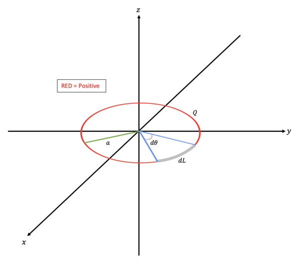
- A ring of evenly distributed charge of radius [math]\displaystyle{ a }[/math] is centered on the origin in the xy-plane. The ring has a total charge [math]\displaystyle{ Q }[/math]. Show that the Electric Field due to this ring is 0 at the origin.
- Solution:
- The Electric Field due to a point charge is given by:
- [math]\displaystyle{ \mathbf{E} = \frac{1}{4 \pi \epsilon_{0}} \frac{|Q|}{| \mathbf{r} - \mathbf{r}^{'} |^{2}} \frac{\mathbf{r} - \mathbf{r}^{'}}{| \mathbf{r} - \mathbf{r}^{'} |} }[/math]
- This equation is equivalent to the formula presented in the Mathematical Model. The reason it looks so different is due to a few assumptions in the mathematical model that we have stopped using:
- The source charge is located at the origin (our ring of charge is around the origin)
- The distance between the source charge and the observing location is simply expressed as a distance [math]\displaystyle{ r }[/math] (like in the Middling Example). Now, instead we will represent the distance as the magnitude of the difference in position between the source and observer [math]\displaystyle{ \big( | \mathbf{r} - \mathbf{r}^{'} | \big) }[/math].
- Subsequently, our unit vector in the direction of the field [math]\displaystyle{ \big( \hat{\mathbf{r}} \big) }[/math] is not simply expressed as a typical unit vector (like in the middling example). It has now become the vector joining the source and observer divided by the magnitude of this same vector [math]\displaystyle{ \bigg( \frac{\mathbf{r} - \mathbf{r}^{'}}{| \mathbf{r} - \mathbf{r}^{'} |} \bigg) }[/math].
- The Electric Field due to a point charge is given by:
- Another complication this problem presents is:
- Where is the source charge?
- To answer this, notice that the ring has an evenly distributed TOTAL charge [math]\displaystyle{ Q }[/math] and a radius [math]\displaystyle{ a }[/math]. Also, notice that the "source" position is constantly changing as you go around the ring. This issue makes it much more convenient to speak of the line charge DENSITY at a point along the ring instead of the TOTAL charge. This will allow us to treat the ring as many, many little source charges. The line charge density is simply the charge on the line divided by the length of that line (circumference), since the charge is evenly distributed about the ring:
- Another complication this problem presents is:
- [math]\displaystyle{ \rho_{L} = \frac{Q}{2 \pi a} }[/math]
- This allows us to represent a differential amount of source charge as a product of the line charge density and a differential length:
- [math]\displaystyle{ dQ = \rho_{L} dL }[/math]
- The next question is: What is a differential length around the ring?
- The differential length is a differential arc length [math]\displaystyle{ (s = r \theta) }[/math] around the circle dependent on the change in angle:
- [math]\displaystyle{ dL = a d\theta }[/math]
- Therefore:
- [math]\displaystyle{ \begin{align} dQ &= \frac{Q}{2 \pi a} a d\theta \\ &= \frac{Q}{2 \pi} d\theta \\ \end{align} }[/math]
- Therefore:
- Now we can sum each of these differential source charge's contribution to the Electric Field at the origin using an integral:
- [math]\displaystyle{ \mathbf{E} = \int \frac{1}{4 \pi \epsilon_{0}} \frac{\frac{Q}{2 \pi} d\theta}{| \mathbf{r} - \mathbf{r}^{'} |^{2}} \frac{\mathbf{r} - \mathbf{r}^{'}}{| \mathbf{r} - \mathbf{r}^{'} |} }[/math]
- Now we can sum each of these differential source charge's contribution to the Electric Field at the origin using an integral:
- The only things left to find are the generic source position (a vector that can describe the position of each differential source charge along the ring) and the observer location. The observer location is given to us; the origin:
- [math]\displaystyle{ \mathbf{r} = 0\mathbf{i} +0\mathbf{j} + 0\mathbf{k} }[/math]
- The only things left to find are the generic source position (a vector that can describe the position of each differential source charge along the ring) and the observer location. The observer location is given to us; the origin:
- The source position is easiest to describe as a radius from the origin (polar coordinates):
- [math]\displaystyle{ \mathbf{r}^{'} = a \hat{ \mathbf{a}}_{r} }[/math] where [math]\displaystyle{ \hat{\mathbf{a}}_{r} }[/math] is a unit vector in the radial direction
- The source position is easiest to describe as a radius from the origin (polar coordinates):
- Therefore:
- [math]\displaystyle{ \begin{align} \mathbf{r} - \mathbf{r}^{'} &= \big( 0\mathbf{i} +0\mathbf{j} + 0\mathbf{k} \big) - \big( a\hat{ \mathbf{a}}_{r} \big) \\ &= -a\hat{ \mathbf{a}}_{r} \\ |\mathbf{r} - \mathbf{r}^{'}| &= \sqrt{(-a)^{2}} \\ &= a \\ \end{align} }[/math]
- Therefore:
- Plugging these into the Electric Field integral gives:
- [math]\displaystyle{ \begin{align} \mathbf{E} &= \int \frac{1}{4 \pi \epsilon_{0}} \frac{\frac{Q}{2 \pi} d\theta}{a^2} \frac{-a \hat{ \mathbf{a}}_{r}}{a} \\ &= - \int \frac{1}{8 {\pi}^{2} \epsilon_{0}} \frac{Q}{a^2} \hat{ \mathbf{a}}_{r} d\theta \\ &= - \frac{Q}{a^{2} 8 {\pi}^{2} \epsilon_{0}} \int \hat{ \mathbf{a}}_{r} d\theta \\ \end{align} }[/math]
- Plugging these into the Electric Field integral gives:
- [math]\displaystyle{ \theta }[/math] is the angle from the x-axis.
- To integrate over the entire ring, we set the bounds of [math]\displaystyle{ \theta }[/math] as [math]\displaystyle{ [0, 2 \pi) }[/math].
- Also, as of right now, the integral would not evaluate to 0. This is because [math]\displaystyle{ \hat{ \mathbf{a}}_{r} }[/math] has a hidden dependence on [math]\displaystyle{ \theta }[/math]:
- [math]\displaystyle{ \hat{ \mathbf{a}}_{r} = \text{cos}( \theta) \mathbf{i} + \text{sin}( \theta) \mathbf{j} }[/math]
- Plugging this information in gives:
- [math]\displaystyle{ \begin{alignat}{3} \mathbf{E} &= - \frac{Q}{a^{2} 8 {\pi}^{2} \epsilon_{0}} \int_{0}^{2 \pi} \big( \text{cos}( \theta) \mathbf{i} + \text{sin}( \theta) \mathbf{j} \big) d\theta \\ \int_{0}^{2 \pi} \text{cos}( \theta) \mathbf{i} \ d\theta &= 0 \\ \int_{0}^{2 \pi} \text{sin}( \theta) \mathbf{j} \ d\theta &= 0 \\ \end{alignat} }[/math]
- Plugging this information in gives:
- Therefore:
- [math]\displaystyle{ \mathbf{E} = 0 }[/math] at the origin.
- Therefore:
Non-Coulomb Electric Field
Example:
A long solenoid has radius [math]\displaystyle{ R = 0.10 \text{ m} }[/math] and contains 500 turns per meter. The current through the solenoid increases according to [math]\displaystyle{ I(t) = 2.0t \ \text{A} }[/math], where [math]\displaystyle{ t }[/math] is in seconds.
Find the induced non-Coulomb electric field [math]\displaystyle{ \vec{E}_{nc} }[/math] at [math]\displaystyle{ r = 0.20 \text{ m} }[/math] outside the solenoid.
Solution
Step 1: Find magnetic field inside the solenoid
[math]\displaystyle{ B(t) = \mu_0 n I(t) }[/math]
[math]\displaystyle{ B(t) = (4\pi \times 10^{-7})(500)(2t) }[/math]
[math]\displaystyle{ B(t) = 1000\pi \times 10^{-7} t }[/math]
[math]\displaystyle{ B(t) = 4\pi \times 10^{-4} t \ \text{T} }[/math]
Step 2: Take derivative of magnetic field
[math]\displaystyle{ \frac{dB}{dt} = 4\pi \times 10^{-4} \ \text{T/s} }[/math]
Step 3: Apply Faraday’s Law
[math]\displaystyle{ \oint \vec{E}_{nc} \cdot d\vec{\ell} = -\frac{d\Phi_B}{dt} }[/math]
Magnetic flux:
[math]\displaystyle{ \Phi_B = B \pi R^2 }[/math]
[math]\displaystyle{ \frac{d\Phi_B}{dt} = \frac{dB}{dt} \pi R^2 }[/math]
Left side of loop:
[math]\displaystyle{ \oint \vec{E}_{nc} \cdot d\ell = E_{nc}(2\pi r) }[/math]
Equate both sides:
[math]\displaystyle{ E_{nc}(2\pi r) = -\frac{dB}{dt} \pi R^2 }[/math]
Solve for the induced field:
[math]\displaystyle{ E_{nc} = -\frac{1}{2}\frac{dB}{dt}\frac{R^2}{r} }[/math]
Step 4: Substitute numerical values
[math]\displaystyle{ E_{nc} = -\frac{1}{2}(4\pi \times 10^{-4}) \frac{(0.10)^2}{0.20} }[/math]
[math]\displaystyle{ E_{nc} = -9 \times 10^{-6} \ \text{V/m} }[/math]
Final value:
[math]\displaystyle{ E_{nc} = -3.14 \times 10^{-5} \ \text{V/m} }[/math]
(The negative sign indicates direction.)
Note: Notice how we worked the example by using other factors, such as the radius of the solenoid itself and the B-field the solenoid creates, to find the induced electric field. Non-Coulomb electric fields come only as a result of changing B fields, which is why magnetic flux is taken into account.
Connectedness
The real world applications of electric fields are endless. Here are some:
- Electric Motors:
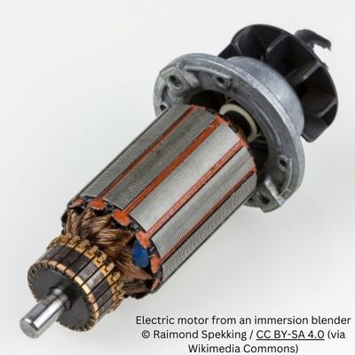
- Electric motors convert Electrical Energy into Mechanical Energy through Electric Fields. Whenever electric motors are turned on, Electric Fields are generated. This is because in order to turn an electric motor, an Electric Field must first be generated, which then generates a Magnetic Field, thus making the motor spin. Electric motors are used in cars, elevators, fans, refrigerators, and many more applications.
- Computers:
- Computers use circuits, electric fans, and transistors to work. All of these use Electric Fields to push charge through a circuit, spin fans, and allow logic to be implemented in electronics.
- Painting:
- Electric Fields are also used in some paintings. The Electric Field generates charges on the surface of the material being painted on, and an opposite charge is generated on the paint. Paint that touches the material sticks, and excess paint falls off to go back into the system.
- Cancer Treatment:
- Recently, weak Electric Fields have been used to kill cancer cells. This treatment works best for brain and breast cancers, and it has no effect on normal cells. In lab and animal tests, this treatment killed cancer cells of every type tested; however, this is still a developing treatment.
- Military and Defense:
- Electric Fields are commonly used in various weapons platforms. Weapons used to rely primarily on explosives; however, electric weapons use stored electrical energy to attack targets. There are two general types: directed-energy weapons (DEWs) and electromagnetic (EM) weapons. DEWs include lasers, radio frequency weapons, and more. EM weapons include rail guns, coil guns, etc. For example, rail guns use EM force to launch high velocity projectiles at a target. They work by using very high electrical currents to induce magnetic fields that accelerate a projectile to extremely high speeds (up to Mach 6).
- Air Purifiers & Printers:
- Electrostatic precipitators in air filters use Electric Fields to charge dust and pollutant particles so they can be trapped on oppositely charged plates. Similarly, laser printers and photocopiers use carefully controlled Electric Fields to attract toner particles onto specific regions of paper.
- Lightning & Weather Phenomena:
- Lightning is a massive discharge caused by built-up Electric Fields between clouds and the ground. Electric Fields also drive corona discharge, St. Elmo’s fire, and charge separation processes inside thunderstorms.
- Touchscreens:
- Capacitive touchscreens (found in phones, tablets, laptops) rely on changes in local Electric Fields when your finger — a conductor — touches the screen. The device senses these field changes to determine your touch location.
- Biology & Nerve Signals:
- Nerve cells communicate using voltage differences and Electric Fields along axons and cell membranes. These electric potentials allow neurons to fire signals that control movement, thought, and sensory perception.
- Sensors & Medical Devices:
- Devices like ECG and EEG use tiny Electric Fields generated by the heart and brain to monitor biological activity. Electric Fields also drive electrophoresis, a technique used in DNA and protein analysis.
- Plasma Globes & Neon Signs:
- Plasma globes and neon tubes use strong Electric Fields to ionize gases. The accelerated electrons collide with gas atoms, producing light — a vivid example of how electric fields interact with matter.
History
Electric Fields are created by Electric charges. The original discovery of the Electric charge is not explicitly known, but in 1675 the esteemed chemist Robert Boyle, known for Boyle's Law, discovered the attraction and repulsion of certain particles in a vacuum. Almost 100 years later in the 18th century, the American Benjamin Franklin first coined the phrases 'positive' and 'negative' (later developed into proton and electron) for these particles with attractive and repulsive properties. Finally, in the 19th century Michael Faraday utilized his Electrolysis process to discover the discrete nature of Electric charge.
See also
The ability to understand Electric Fields helps set the basis for the introduction to Electric Force (as we discussed [math]\displaystyle{ \mathbf{F} = q\mathbf{E} }[/math] ). The introduction of Electric Force will attach the specific charge of the particles with the Electric Field that they produce, resulting in the Electric Force. Electric Force will lay the ground work for understanding the force that particles have in different systems and environments, and eventually lead to the introduction of Magnetic Force. The understanding of Electric Fields is a doorway into many various fields, only some of which will be covered in Physics 2212. The fundamental understanding of Electric Fields will prove to be very important further along when Magnetic Fields are introduced, as they share many qualities. The understanding of Electric and Magnetic Fields will be used throughout the semester to learn about various Electromagnetic concepts, and ultimately to understanding and apply Maxwell's Equations. Please see related topics:
Further reading
External links
References
- OpenStax Volume on Electricity and Magnetism
- Hayt & Buck 9th Edition Engineering Electromagnetics
- Matter and Interactions<be>
Old Simulation Code
   ###--Create Electric Field Lines of a Positive Charge at the Origin--###
   #==============================================================#
   #---Import statements for VPython---#
   from __future__ import division
   from visual import *
   #---Import function used to find combinations---#
   from itertools import combinations
   #==============================================================#
   #---Create scene---#
   scene.center = vector(0,0,0)  #-Position of source charge-#
   scene.height = 800  #-Set height of frame of scene-#
   scene.width = 800  #-Set width of frame of scene-#
   scene.range = 4  #-Set range of scene-#
   scene.userzoom = 1  #-Allow user to zoom in/out: CTRL & move in/out on trackpad-#
   scene.userspin = 1  #-Allow user to rotate camera angle: SHIFT & OPTION & move around on track pad-#
   #==============================================================#
   #---Specify point charge attributes---#
   sourceCharge = 3*10**(-11)  #-Coulombs of charge-#
   sourcePos = vector(0,0,0) #-Position of source charge-#
   ###--Modeling source point charge as a sphere with radius 0.1 meters--###
   sourceObj = sphere(pos = sourcePos, radius = 0.1, color = color.cyan)
   #==============================================================#
   #---Set range (0 to 3) and possible inputs for the coordinates (0.5 step)---#
   ###--Many of the same number included to allow for combinations such as (1,1,1).
       #The itertools.combinations function will only use each element of the...
       #list once, starting from the beginning.
       #Repeating each coordinate many times with intermixing, grants...
       #all combinations of points, with repeats however.
       #Later, a for loop will be used to eliminate repeats.
       #This can be optimized later if need be.---------------###
   posXYZ = [0, -0.5, 1, -1.5, 2, -2.5, 3,
             0, 0.5, -1, 1.5, -2, 2.5, -3,
             0, -0.5, 1, -1.5, 2, -2.5, 3,
             0, 0.5, -1, 1.5, -2, 2.5, -3,
             0, -0.5, 1, -1.5, 2, -2.5, 3,
             0, 0.5, -1, 1.5, -2, 2.5, -3,
             0, -0.5, 1, -1.5, 2, -2.5, 3,
             0, 0.5, -1, 1.5, -2, 2.5, -3,
             0, -0.5, 1, -1.5, 2, -2.5, 3,
             0, 0.5, -1, 1.5, -2, 2.5, -3,
             0, -0.5, 1, -1.5, 2, -2.5, 3,
             0, 0.5, -1, 1.5, -2, 2.5, -3]
   #==============================================================#
   #---Create combinations of points (x,y,z) for later use---#
       ###--prelimPoints will be a list of tuples of tuples--##
           #ie: [((,,),(,,),(,,),(,,)) , ((,,),(,,)) ,..., ((,,),(,,))]
   prelimPoints = [tuple(combinations(posXYZ, 3))]
   ###--Pull the points out of the grouping tuples and add them to a...
       #new list alphaPoints------------------------###
   alphaPoints = []
   for groupingTuple in prelimPoints:
       for XYZ in groupingTuple:
           if XYZ not in alphaPoints:  #-Check for repeat (x,y,z)-#
               alphaPoints.append(XYZ)
           ##--The negative of this tuple may not be in the combinations:
               #check to see-------------##
           first = -XYZ[0]
           second = -XYZ[1]
           third = -XYZ[2]
           negXYZ = (first, second, third)
           if negXYZ not in alphaPoints:
               alphaPoints.append(negXYZ)
           ##--Swap x and z coordinates for futher combination checking--##
           first = XYZ[2]
           second = XYZ[1]
           third = XYZ[0]
           reverseXYZ = (first, second, third)
           if reverseXYZ not in alphaPoints:
               alphaPoints.append(reverseXYZ)
           ##--The negative of the x and z coordinate swap may not be in...
               #the combinations: check to see---------##
           first = -XYZ[2]
           second = -XYZ[1]
           third = -XYZ[0]
           reverseXYZneg = (first, second, third)
           if reverseXYZneg not in alphaPoints:
               alphaPoints.append(reverseXYZneg)
           ##--Make x [3], y [0], and z [1] to check for more combinations--##
           first = XYZ[1]
           second = XYZ[2]
           third = XYZ[0]
           shiftedXYZ = (first, second, third)
           if shiftedXYZ not in alphaPoints:
               alphaPoints.append(shiftedXYZ)
           ##--The negative of the shifted XYZ may not be in the combinations:
               #check to see---------------##
           first = -XYZ[1]
           second = -XYZ[2]
           third = -XYZ[0]
           shiftedXYZneg = (first, second, third)
           if shiftedXYZneg not in alphaPoints:
               alphaPoints.append(shiftedXYZneg)
   ###--------This should be enough recombining---------###
   #================================================================#
   #---Create a new list of tuples that contain the points, magnitude,...
       #and direction (betaPoints)-----------#
           #ie: [((x,y,z), mag((x,y,z)), norm((x,y,z))),...]
   betaPoints = []
   for XYZ in alphaPoints:
       Mag = mag(XYZ)
       Dir = norm(XYZ)
       betaPoints.append((XYZ, Mag, Dir))
   #================================================================#
   #---Sort the tuples based on their magnitudes from least to greatest...
      #using sorted().
           #key = lamda x: x[1] tells the sorted function to sort the tuples...
               #based on their second component...their magnitudes--------#
   charliePoints = sorted(betaPoints, key = lambda x: x[1])
   #================================================================#
   #---Calculate parts of electric field equation:
       #E = 1/(4*pi*epsilon0) * Q/(magnitude)**2
   epsilonO = 8.854*(10**(-12)) #-N*(m/C)**2-#
   k = 1/(4*pi*(epsilonO)) #-N*(m/C)**2-#
   chargeContri = k*sourceCharge #-N*(m**2/C)-#
   #================================================================#
   #---Loop through points and find mag of electric field:
       #add it to a new list with the existing tuple info-------#
   deltaPoints = []
   for XYZ in charliePoints:
       try:  ###-Avoid divide by 0 error in (x,y,z) = (0,0,0)-###
           magEfield = chargeContri*(1/(XYZ[1])**2)
       except:
           magEfield = 0
       tupEfield = (XYZ[0], XYZ[1], XYZ[2], magEfield)
       deltaPoints.append(tupEfield)
   #================================================================#
   #---Loop through points and create an arrow at that point proportional in...
       #length to the magnitude of the electric field there.
       #Also, the arrow points in the direction of the electric field there.
       #Color coding is based on 0.25 meter increments:
           #stronger field = redder; weaker field = blue
   for XYZ in deltaPoints:
       if XYZ[1] <= 0.25:
           lengthP = XYZ[3]*0.5
           arroW = arrow(pos=vector(XYZ[0]), axis=XYZ[2],
                         color = vector(1.000, 0.000, 0.000),
                         length = lengthP,
                         headwidth = lengthP*0.2,
                         headlength = lengthP*0.25)
       elif XYZ[1] <= 0.5:
           lengthP = XYZ[3]*0.7
           arroW = arrow(pos=vector(XYZ[0]), axis=XYZ[2],
                         color = vector(1.000, 0.200, 0.000),
                         length = lengthP,
                         headwidth = lengthP*0.2,
                         headlength = lengthP*0.25)
       elif XYZ[1] <= 1:
           lengthP = XYZ[3]*0.9
           arroW = arrow(pos=vector(XYZ[0]), axis=XYZ[2],
                         color = vector(1.000, 0.300, 0.000),
                         length = lengthP,
                         headwidth = lengthP*0.2,
                         headlength = lengthP*0.25)
       elif XYZ[1] <= 1.25:
           lengthP = XYZ[3]*1.1
           arroW = arrow(pos=vector(XYZ[0]), axis=XYZ[2],
                         color = vector(1.000, 0.400, 0.000),
                         length = lengthP,
                         headwidth = lengthP*0.2,
                         headlength = lengthP*0.25)
       elif XYZ[1] <= 1.5:
           lengthP = XYZ[3]*1.3
           arroW = arrow(pos=vector(XYZ[0]), axis=XYZ[2],
                         color = vector(1.000, 0.500, 0.000),
                         length = lengthP,
                         headwidth = lengthP*1,
                         headlength = lengthP*1)
       elif XYZ[1] <= 1.75:
           lengthP = XYZ[3]*1.5
           arroW = arrow(pos=vector(XYZ[0]), axis=XYZ[2],
                         color = vector(1.000, 0.600, 0.000),
                         length = lengthP,
                         headwidth = lengthP*1,
                         headlength = lengthP*1)
       elif XYZ[1] <= 2:
           lengthP = XYZ[3]*1.7
           arroW = arrow(pos=vector(XYZ[0]), axis=XYZ[2],
                         color = vector(1.000, 0.700, 0.000),
                         length = lengthP,
                         headwidth = lengthP*1,
                         headlength = lengthP*1)
       elif XYZ[1] <= 2.25:
           lengthP = XYZ[3]*1.9
           arroW = arrow(pos=vector(XYZ[0]), axis=XYZ[2],
                         color = vector(1.000, 0.800, 0.000),
                         length = lengthP,
                         headwidth = lengthP*1,
                         headlength = lengthP*1)
       elif XYZ[1] <= 2.5:
           lengthP = XYZ[3]*2.1
           arroW = arrow(pos=vector(XYZ[0]), axis=XYZ[2],
                         color = vector(1.000, 0.900, 0.000),
                         length = lengthP,
                         headwidth = lengthP*1,
                         headlength = lengthP*1)
       elif XYZ[1] <= 2.75:
           lengthP = XYZ[3]*2.3
           arroW = arrow(pos=vector(XYZ[0]), axis=XYZ[2],
                         color = vector(1.000, 1.000, 0.000),
                         length = lengthP,
                         headwidth = lengthP*1,
                         headlength = lengthP*1)
       else:
           lengthP = XYZ[3]*2.5
           arroW = arrow(pos=vector(XYZ[0]), axis=XYZ[2],
                         color = color.blue,
                         length = lengthP,
                         headwidth = lengthP*1,
                         headlength = lengthP*1)