Vectors: Difference between revisions
Msridhar30 (talk | contribs) No edit summary |
No edit summary |
||
| (286 intermediate revisions by 14 users not shown) | |||
| Line 1: | Line 1: | ||
'''Aditya Verma – Fall 2025''' | |||
==Vectors and Units Introduction== | |||
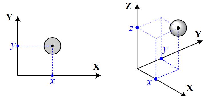
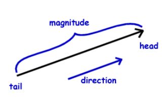
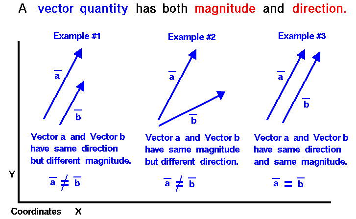
Vectors and units are core tools for describing the physical world in a precise, quantitative way. A vector is a quantity that has both **magnitude** (how big) and **direction** (which way). Many important physical quantities are vectors: displacement, velocity, acceleration, and force all need both size and direction to be completely specified. By representing these quantities as vectors, we can keep track of how they combine, cancel, and interact in one, two, or three dimensions. | |||
Units, meanwhile, tell us **what** we are measuring. A number by itself has no physical meaning until we attach a unit such as meters (m), seconds (s), or newtons (N). Consistent use of units helps us spot mistakes, compare results, and communicate clearly. Together, vectors and units allow scientists, engineers, and programmers to build models that match real-world behavior and to carry out calculations that remain physically meaningful. | |||
In physics and engineering, vectors show up whenever we track motion, balance forces, or work with fields such as electric and magnetic fields. In computer science and related fields, vectors appear in computer graphics, simulations, game physics, machine learning, and data representation. Units ensure that all of these computations line up with real measurements rather than just abstract numbers. A strong grasp of both vectors and units is essential for solving problems, interpreting formulas, and understanding how different parts of a system relate to each other. | |||
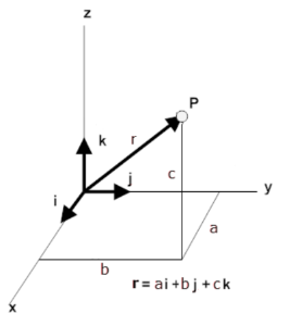
Vectors are usually written using boldface letters or an arrow, such as '''v''' or <math>\vec{v}</math>. You may also see a vector written as a directed segment like <math>\overrightarrow{AB}</math>. Common vector quantities include displacement, velocity, force, and acceleration. Units provide the scale for these quantities and are based on standard systems like SI. For example, meters (m) measure length, kilograms (kg) measure mass, seconds (s) measure time, and newtons (N) measure force. | |||
[[File:2d3dvec.png|2D vector vs 3D vector]][[File:smallvector.png]] | |||
==Unit Vector== | |||
A **unit vector** is a vector whose magnitude is exactly 1 (one unit) but that still points in a particular direction. Unit vectors are useful for representing direction independently of size. They are often used to define coordinate directions (such as the x, y, and z axes) and to rewrite any vector as “magnitude × direction.” | |||
[[File:unitvecexp.png]] | |||
==Magnitude== | |||
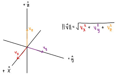
The **magnitude** of a vector is the length or size of the vector. For a vector <math>\vec{v}</math>, the magnitude is written as <math>|\vec{v}|</math>. Magnitude is always a non-negative scalar. In 2D and 3D, it is usually computed with the Pythagorean theorem, using the vector’s components. | |||
[[File:vec3.png]] | |||
== | ==Direction== | ||
The **direction** of a vector describes how it is oriented in space. It can be specified relative to axes (such as the angle from the positive x-axis), using unit vectors, or using geometric descriptions (like “30° above the horizontal” or “to the south”). | |||
[[File:directionvec.png]] | |||
[[File:vec10.png]] | |||
==Addition and Subtraction== | |||
Vectors can be added or subtracted to form new vectors. Geometrically, we often use the **head-to-tail method** or the **parallelogram rule**. In component form, vector addition and subtraction are done by adding or subtracting corresponding components. | |||
[[File:vec4.png]] | |||
==Scalar Multiplication== | |||
**Scalar multiplication** means multiplying a vector by a scalar (a regular number). This produces a new vector in the same or opposite direction, but with its magnitude scaled by the scalar. This is used to stretch, shrink, or reverse vectors in many physical and mathematical problems. | |||
[[File:vec5.png]] | |||
==Dot Product== | |||
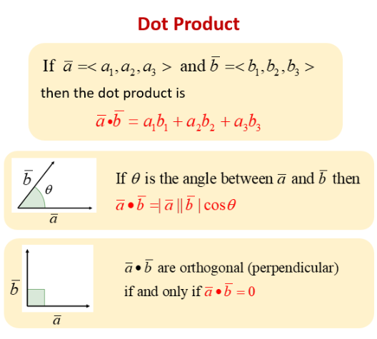
The **dot product** (or scalar product) of two vectors produces a scalar. It can be written in terms of components or in terms of magnitudes and the cosine of the angle between the vectors. Dot products are used to find angles between vectors, project one vector onto another, and calculate physical quantities such as work. | |||
[[File:vec7.png]] | |||
==Cross Product== | |||
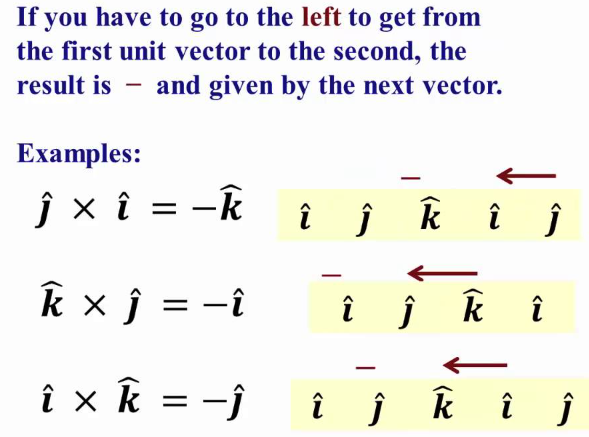
The **cross product** (or vector product) of two vectors in 3D produces a new vector that is perpendicular to both original vectors. Its magnitude equals the product of the magnitudes of the two vectors times the sine of the angle between them. Cross products appear in torque, angular momentum, and magnetic force, among other topics in rotational and field-based physics. | |||
[[File:vec8.png]] | |||
The | For two vectors <math>\vec{A}</math> and <math>\vec{B}</math>, the magnitude of the cross product is | ||
<math>|\vec{A}\times\vec{B}| = |\vec{A}|\;|\vec{B}|\sin(\theta)</math>, | |||
where <math>\theta</math> is the angle between them. The direction follows the **right-hand rule**. | |||
Some useful properties of the cross product: | |||
* It is **not commutative**: <math>\vec{A}\times\vec{B} \neq \vec{B}\times\vec{A}</math>. In fact, <math>\vec{A}\times\vec{B} = -(\vec{B}\times\vec{A})</math>. | |||
* It is **distributive** over addition: <math>\vec{A}\times(\vec{B} + \vec{C}) = \vec{A}\times\vec{B} + \vec{A}\times\vec{C}</math>. | |||
* The cross product of a vector with itself is zero: <math>\vec{A}\times\vec{A} = \vec{0}</math>, since the angle between a vector and itself is 0 and <math>\sin(0) = 0</math>. | |||
==SI Units== | |||
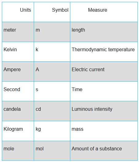
The **International System of Units (SI)** is the main measurement system used in science and engineering. It specifies seven base units from which all other units are built: | |||
* meter (m) – length | |||
* kilogram (kg) – mass | |||
* second (s) – time | |||
* ampere (A) – electric current | |||
* kelvin (K) – temperature | |||
* mole (mol) – amount of substance | |||
* candela (cd) – luminous intensity | |||
All physical vector quantities you encounter in this class will use combinations of these units. | |||
[[File:vec11.png]] | |||
==Derived Units== | |||
**Derived units** are units formed by combining base units through multiplication and division. For example: | |||
* newton (N) = kg·m/s<sup>2</sup> (force) | |||
* joule (J) = N·m (energy) | |||
* watt (W) = J/s (power) | |||
These units describe more complex physical quantities but are always traceable back to the SI base units. | |||
==Conversion== | |||
**Unit conversion** means changing a quantity from one set of units to another while representing the same physical amount. For example, converting from centimeters to meters or from kilometers per hour to meters per second. In multi-step physics problems, careful unit conversion is essential to avoid errors and to match the units expected in formulas. | |||
==Applications== | |||
Vectors and units appear in many areas: | |||
* **Physics:** describing motion, forces, fields (electric, magnetic, gravitational), and momentum. | |||
* **Engineering:** analyzing structures, designing mechanical systems, working with fluid flow, and modeling electrical circuits. | |||
* **Computer Graphics:** representing positions, directions, lighting, and transformations in 2D and 3D scenes. | |||
* **Navigation:** expressing position, velocity, and direction in GPS systems and for aircraft or ships. | |||
Understanding how vectors and units work together lets us build accurate models and interpret real-world data correctly. | |||
_________________________________________________________________________________________________________________________________________________________________________________________________________________________________________________________________________________________________________ | |||
==What is a Vector?== | |||
In | In mathematics and physics, a **vector** is a quantity that has both a magnitude and a direction. | ||
In coordinates, we often write a vector as a list of components. For example, in a 3D coordinate system, we might write: | |||
<math>\vec{v} = \langle v_x, v_y, v_z \rangle</math> | |||
Here: | |||
* <math>v_x</math> is the x-component of the vector, | |||
* <math>v_y</math> is the y-component, | |||
* <math>v_z</math> is the z-component. | |||
A vector can also be written as a boldface letter, such as '''a''', or with an arrow, like <math>\vec{a}</math>. The specific letter used often reflects the quantity: <math>\vec{v}</math> for velocity, <math>\vec{r}</math> for position, etc. Individual components of a vector are written with subscripts, such as <math>c_x</math> or <math>q_y</math>. | |||
====Example of a Simple Vector==== | |||
--[[ | <math>\vec{v} = \langle 1, 0, 0 \rangle</math> | ||
This vector has magnitude 1 and points along the positive x-direction in 3D space. | |||
===Magnitude=== | |||
The **magnitude** (or length) of a vector tells us how large the vector is. | |||
We denote the magnitude of <math>\vec{v}</math> using vertical bars: | |||
<math>|\vec{v}|</math>. You might also see notations such as <math>\overline{v}</math> or <math>\lVert\vec{v}\rVert_2</math> (the Euclidean norm). | |||
In a 3D system, if | |||
<math>\vec{v} = \langle v_x, v_y, v_z \rangle</math>, | |||
then its magnitude is | |||
<math>\lVert \vec{v} \rVert = \sqrt{v_x^2 + v_y^2 + v_z^2}.</math> | |||
More generally, in n dimensions, | |||
<math>\lVert \vec{v} \rVert = \sqrt{v_1^2 + v_2^2 + \cdots + v_n^2}.</math> | |||
The magnitude carries the units of the quantity being represented. For example, the magnitude of a velocity vector is speed and has units of m/s. | |||
Note that a vector does not always represent a literal “arrow in space” between two locations. Often, a vector describes a property at a single point (like electric field at a location) or in an abstract space, even though the mathematics is the same. | |||
[[File:IMG_0325613.jpg|400px|Image: 400 pixels]] | |||
====Unit Vector==== | |||
If we divide a nonzero vector by its magnitude, we obtain a **unit vector** in the same direction: | |||
<math>\hat{v} = \frac{\vec{v}}{\lVert \vec{v} \rVert}</math>. | |||
For example, if <math>\vec{v} = \langle v_x, v_y, v_z \rangle</math>, then | |||
<math>\hat{v} = \frac{1}{\lVert\vec{v}\rVert}\langle v_x, v_y, v_z \rangle.</math> | |||
Unit vectors are written with a “hat,” such as <math>\hat{v}</math>. In many coordinate systems, there are standard unit vectors. In 3D Cartesian coordinates, the unit vectors along the axes are | |||
<math>\hat{x} = \langle 1, 0, 0 \rangle, \quad \hat{y} = \langle 0, 1, 0 \rangle, \quad \hat{z} = \langle 0, 0, 1 \rangle.</math> | |||
Other coordinate systems use different unit vectors, like <math>\hat{r}</math> and <math>\hat{\theta}</math> in polar coordinates. | |||
===Direction=== | |||
The **direction** of a vector tells us which way it points. | |||
In 2D, we usually measure direction by an angle from the positive x-axis. For a vector <math>\vec{v} = \langle v_x, v_y \rangle</math>, the direction angle <math>\theta</math> can be computed as | |||
<math>\theta = \arctan\left(\frac{v_y}{v_x}\right)</math>, | |||
keeping track of the correct quadrant. | |||
===Simple Examples of Vector Quantities=== | |||
====Position==== | |||
A point’s position can be written as a vector. If we have two position vectors, subtracting them gives the **relative position** from one point to the other. The magnitude of this relative position vector gives the straight-line distance between the two points. A common special case is the position relative to the origin, where the origin is at <math>\langle 0,0,0\rangle</math>. | |||
====Velocity==== | |||
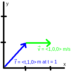
**Velocity** is a vector that describes how fast and in what direction an object moves. Its magnitude is the **speed**, and it is usually measured in m/s. The velocity vector can be found by differentiating the position vector with respect to time. | |||
For example, let <math>\vec{r}(t) = \langle t, 1, 0 \rangle\ \text{m}</math>. Then the velocity is | |||
<math>\vec{v}(t) = \frac{d\vec{r}}{dt} = \langle 1, 0, 0 \rangle\ \text{m/s}.</math> | |||
The speed is the magnitude of <math>\vec{v}</math>, which in this case is 1 m/s. | |||
[[File:Velwiki.png]] | |||
====Weight (Force of Gravity)==== | |||
Weight is the gravitational force acting on an object; it is a vector that typically points downward. We often write the gravitational force as <math>\vec{F_g}</math>. In a coordinate system where +y is upward, we can write: | |||
<math>\vec{F_g} = \langle 0, -mg, 0 \rangle,</math> | |||
where <math>m</math> is the mass of the object and <math>g = 9.8~\text{m/s}^2</math> is the magnitude of the gravitational field near Earth’s surface. The magnitude <math>|\vec{F_g}| = mg</math> is the weight of the object. | |||
===Visually Representing Vectors=== | |||
Vectors are often drawn as **arrows**. The length of the arrow represents the magnitude, and the direction of the arrow shows which way the vector points. If a vector is tied to a particular location, the tail of the arrow is drawn at that point. | |||
The example below shows a velocity vector for a ball moving to the right at 5 m/s. | |||
[[File:Vectorvisualrepresentation.png]] | |||
==Vector Operations== | |||
We can perform several operations on vectors, both with other vectors and with scalars. These operations are used constantly in physics and engineering. To keep the notation simple, we will describe them for 3D vectors, but they generalize naturally to higher dimensions. | |||
===Addition=== | |||
For vectors <math>\vec{a} = \langle a_x, a_y, a_z \rangle</math> and <math>\vec{b} = \langle b_x, b_y, b_z \rangle</math>, | |||
<math>\vec{a} + \vec{b} = \langle a_x + b_x,\; a_y + b_y,\; a_z + b_z \rangle.</math> | |||
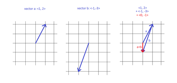
Geometrically, we place the tail of <math>\vec{b}</math> at the head of <math>\vec{a}</math>. The vector from the tail of <math>\vec{a}</math> to the head of <math>\vec{b}</math> is the **resultant** <math>\vec{a} + \vec{b}</math>. | |||
[[File:Vectoraddition.png|600px]] | |||
===Subtraction=== | |||
Vector subtraction can be viewed as adding the negative of a vector. We have | |||
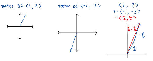
<math>\vec{a} - \vec{b} = \vec{a} + (-\vec{b}) = \langle a_x - b_x,\; a_y - b_y,\; a_z - b_z \rangle.</math> | |||
Component-wise, we subtract each component of <math>\vec{b}</math> from the corresponding component of <math>\vec{a}</math>. | |||
[[File:IMG_0326.jpg|500px|Image: 500 pixels]] | |||
===Multiplication by Scalar=== | |||
If <math>k</math> is a scalar and <math>\vec{a} = \langle a_x, a_y, a_z \rangle</math>, then | |||
<math>k \vec{a} = \langle k a_x,\; k a_y,\; k a_z \rangle.</math> | |||
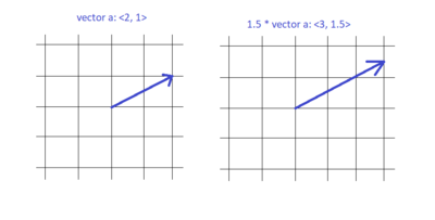
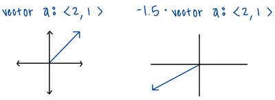
Multiplying by a positive scalar changes the magnitude but keeps the direction the same. Multiplying by a negative scalar flips the direction as well. | |||
[[File:Vectorscalarmultiplication.png|400px]] [[File:IMG_0327.jpg|400px|Image: 400 pixels]] | |||
===Division by Scalar=== | |||
Dividing a vector by a nonzero scalar is equivalent to multiplying by its reciprocal: | |||
<math>\frac{\vec{a}}{k} = \langle \frac{a_x}{k},\; \frac{a_y}{k},\; \frac{a_z}{k} \rangle.</math> | |||
This operation shrinks or enlarges the vector’s magnitude while preserving (or reversing, if k is negative) its direction. | |||
===Dot Product (also called Scalar Product)=== | |||
For <math>\vec{a} = \langle a_x, a_y, a_z \rangle</math> and <math>\vec{b} = \langle b_x, b_y, b_z \rangle</math>, the dot product is | |||
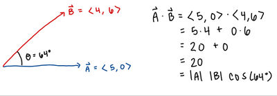
<math>\vec{a}\cdot\vec{b} = a_x b_x + a_y b_y + a_z b_z.</math> | |||
The result is a scalar. The dot product measures how much two vectors “line up” with each other. A key property is | |||
<math>\vec{a}\cdot\vec{b} = |\vec{a}|\;|\vec{b}|\cos(\theta),</math> | |||
where <math>\theta</math> is the angle between <math>\vec{a}</math> and <math>\vec{b}</math>. If the dot product is zero, the vectors are perpendicular. | |||
[[File:IMG_0328.jpg|400px|Image: 400 pixels]] | |||
===Cross Product (also called Vector Product)=== | |||
One component-based definition of the cross product (the one often found on formula sheets) is: | |||
<math>\vec{a} \times \vec{b} = \langle a_yb_z - a_zb_y,\; a_zb_x - a_xb_z,\; a_xb_y - a_yb_x \rangle.</math> | |||
You may also see it written as | |||
<math>\vec{a} \times \vec{b} = (a_yb_z - a_zb_y)\hat{i} - (a_zb_x - a_xb_z)\hat{j} + (a_xb_y - a_yb_x)\hat{k}.</math> | |||
Although this looks complicated, the key idea is that the cross product of two 3D vectors is a new vector that is orthogonal to both of them. The order matters: changing the order flips the sign. | |||
A common way to remember the formula is through the determinant of a 3×3 matrix: | |||
<math>\begin{vmatrix} | |||
\hat{i} & \hat{j} & \hat{k} \\ | |||
a_x & a_y & a_z \\ | |||
b_x & b_y & b_z | |||
\end{vmatrix}.</math> | |||
You can expand this determinant using cofactor expansion. Remember that the <math>\hat{j}</math> term has a minus sign. | |||
[[File:Expansionbyminors.png|400px]] | |||
You can also use online tools or videos to check your work: | |||
* Cross product step-by-step calculator: [https://www.symbolab.com/solver/vector-cross-product-calculator https://www.symbolab.com/solver/vector-cross-product-calculator] | |||
* Video explanation: [https://www.youtube.com/watch?v=e9T5p_Jwv5c https://www.youtube.com/watch?v=e9T5p_Jwv5c] | |||
The magnitude of the cross product satisfies | |||
<math>|\vec{a}\times\vec{b}| = |\vec{a}|\;|\vec{b}|\sin(\theta)</math>, | |||
where <math>\theta</math> is the angle between <math>\vec{a}</math> and <math>\vec{b}</math>. Its direction is perpendicular to the plane of <math>\vec{a}</math> and <math>\vec{b}</math> and is chosen using the [[Right Hand Rule]]. In 2D, the usual cross product is not defined. | |||
<b>For more mathematically-advanced students</b>, we can connect this to linear algebra. Let <math>A \in \mathbb{R}^{m \times n}</math> be a matrix, and consider its **null space**: | |||
<math>\operatorname{Null}(A) = \{ \vec{v} \in \mathbb{R}^n \mid A\vec{v} = \vec{0} \}.</math> | |||
The null space is the set of all vectors that are orthogonal to every row of <math>A</math>. Writing the rows as <math>\vec{a}_1,\ldots,\vec{a}_m</math>, the equation <math>A\vec{v}=\vec{0}</math> expands to | |||
<math>\begin{bmatrix}\vec{a}_1 \\ \vec{a}_2 \\ \vdots \\ \vec{a}_m\end{bmatrix}\vec{v} = \begin{bmatrix}\vec{a}_1 \cdot \vec{v} \\ \vec{a}_2 \cdot \vec{v} \\ \vdots \\ \vec{a}_m \cdot \vec{v}\end{bmatrix} = \begin{bmatrix}0 \\ 0 \\ \vdots \\ 0\end{bmatrix}.</math> | |||
So every vector in the null space is perpendicular to each row, and therefore to the whole row space. | |||
For two vectors <math>\vec{a}, \vec{b} \in \mathbb{R}^3</math> that are not multiples of each other, think of them as the rows of a 2×3 matrix <math>A</math>. The null space of <math>A</math> consists of all vectors orthogonal to both <math>\vec{a}</math> and <math>\vec{b}</math>. The cross product <math>\vec{a}\times\vec{b}</math> is (up to scaling and orientation) the unique nonzero vector in this null space once we fix the magnitude and choose a direction using the right-hand rule. This is another way to see why the cross product is perpendicular to both original vectors. In higher dimensions, the null space can have more than one dimension, so there isn’t a single unique “cross product direction” in the same way. | |||
====Another Cross Product Trick==== | |||
Here is a pattern-based way to compute the cross product quickly, using components. | |||
Suppose | |||
<math>\vec{a} = \langle 3, -2, 4 \rangle, \quad \vec{b} = \langle -1, 6, 3 \rangle.</math> | |||
We want <math>\vec{c} = \vec{a} \times \vec{b} = \langle c_x, c_y, c_z \rangle.</math> | |||
Arrange the components vertically and repeat the first component at the bottom: | |||
<math>\begin{vmatrix} | |||
a_x \\ | |||
a_y \\ | |||
a_z \\ | |||
a_x | |||
\end{vmatrix} | |||
= | |||
\begin{vmatrix} | |||
3 \\ | |||
-2 \\ | |||
4 \\ | |||
3 | |||
\end{vmatrix}</math>, | |||
<math>\begin{vmatrix} | |||
b_x \\ | |||
b_y \\ | |||
b_z \\ | |||
b_x | |||
\end{vmatrix} | |||
= | |||
\begin{vmatrix} | |||
-1 \\ | |||
6 \\ | |||
3 \\ | |||
-1 | |||
\end{vmatrix}</math>. | |||
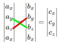
To find <math>c_x</math>, draw an “X” connecting <math>a_y</math> with <math>b_z</math> and <math>a_z</math> with <math>b_y</math>: | |||
[[File:Cx.png]] | |||
Then compute | |||
<math>c_x = a_y b_z - a_z b_y = (-2)(3) - (4)(6) = -6 - 24 = -30.</math> | |||
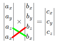
For <math>c_y</math>, use <math>a_z</math> with the bottom <math>b_x</math> and the bottom <math>a_x</math> with <math>b_z</math>: | |||
[[File:Cy.png]] | |||
So | |||
<math>c_y = a_z b_x - a_x b_z = (4)(-1) - (3)(3) = -4 - 9 = -13.</math> | |||
For <math>c_z</math>, connect <math>a_x</math> with <math>b_y</math> and <math>a_y</math> with <math>b_x</math>: | |||
[[File:Cz.png]] | |||
Then | |||
<math>c_z = a_x b_y - a_y b_x = (3)(6) - (-2)(-1) = 18 - 2 = 16.</math> | |||
Thus | |||
<math>\vec{a}\times\vec{b} = \langle -30, -13, 16 \rangle.</math> | |||
With practice, you may not need to draw the X each time and can compute the components directly from the pattern. | |||
==Equations Involving Vector Operations== | |||
You may sometimes encounter equations that mix dot products and cross products. Two useful facts: | |||
<ol> | |||
<li><math>(\vec{w} \times \vec{v}) \cdot \vec{v} = 0</math>, because <math>\vec{w} \times \vec{v}</math> is perpendicular to both <math>\vec{w}</math> and <math>\vec{v}</math>, so its dot product with either original vector is zero.</li> | |||
<li><math>\vec{a} \cdot (\vec{b} \times \vec{c}) = (\vec{a} \times \vec{b}) \cdot \vec{c}</math>. This identity, called the scalar triple product identity, can be useful if one cross product is easier to compute than the other. Note that the cross product part is still order-sensitive, while the dot product is commutative.</li> | |||
</ol> | |||
==Forms== | |||
There are several common ways to describe a vector, all containing the same information. | |||
===Magnitude and Direction Form=== | |||
In this form, we specify: | |||
* The magnitude (length), and | |||
* A description of the direction (cardinal direction, angle, or axis). | |||
For example, “a 5 m vector at 60° above the horizontal” is in magnitude and direction form. This form is intuitive and often used in word problems and real-life descriptions. | |||
===Component Form=== | |||
Here, we break the vector into components along the coordinate axes. In 3D, a vector is written as | |||
<math>\langle a_x, a_y, a_z \rangle.</math> | |||
For example, <math>\langle 2, 0, -3 \rangle</math> means the vector extends 2 units in +x, 0 units in y, and 3 units in -z. Most algebraic operations (like dot and cross products) are done using component form. Programming languages also typically store vectors in this way. | |||
===Unit Vector Form=== | |||
In unit vector form, we write a vector as a combination of unit vectors: | |||
<math>\hat{i}</math>, <math>\hat{j}</math>, <math>\hat{k}</math> or <math>\hat{x}</math>, <math>\hat{y}</math>, <math>\hat{z}</math>. | |||
For instance, the vector <math>\langle 2, 0, -3 \rangle</math> can be written as | |||
<math>2\hat{i} - 3\hat{k}.</math> | |||
Unit vector form and component form contain the same numerical information; they just use different notation. | |||
[[File:Vectorsdifferentforms.png]] | |||
In n dimensions, a vector always needs n numbers to describe it fully. In 3D, magnitude–direction form uses 1 number for magnitude and 2 angles for direction, while component or unit-vector form uses 3 components. | |||
===Converting Between Forms=== | |||
We can move between forms using trigonometry and the Pythagorean theorem. | |||
* For a 2D vector <math>\vec{a} = \langle a_x, a_y \rangle</math>, the magnitude is | |||
<math>|\vec{a}| = \sqrt{a_x^2 + a_y^2}.</math> | |||
* The direction angle from the positive x-axis is | |||
<math>\theta = \tan^{-1}\left(\frac{a_y}{a_x}\right)</math> (with quadrant checks). | |||
* Given magnitude <math>|\vec{a}|</math> and angle <math>\theta</math>, the components are | |||
<math>a_x = |\vec{a}|\cos\theta</math>, | |||
<math>a_y = |\vec{a}|\sin\theta</math>. | |||
==Vectors in VPython== | |||
In VPython (used in GlowScript), vectors are represented by the type <code>vec</code> or <code>vector</code>. The constructor takes three arguments: the x, y, and z components. | |||
Example: | |||
<code>velocity = vec(3, -1, 2)</code> | |||
This creates a vector called <code>velocity</code> with components (3, -1, 2). | |||
In VPython’s default view, +x points to the right, +y points upward, and +z points out of the screen toward the viewer. | |||
===Modifying Vectors=== | |||
You can access or modify individual components using <code>.x</code>, <code>.y</code>, and <code>.z</code>. For example: | |||
<code>velocity.x = 5</code> | |||
changes the x-component from 3 to 5. | |||
===Helpful Vector Functions=== | |||
====Magnitude==== | |||
VPython provides the <code>mag</code> function to compute the magnitude of a vector: | |||
<code> | |||
velocity = vec(3, -1, 2) | |||
speed = mag(velocity) # magnitude of velocity | |||
</code> | |||
====Normalize==== | |||
To obtain a unit vector in the same direction (normalize a vector), use <code>norm</code>: | |||
<code> | |||
v = vec(5, 0, 0) | |||
v_hat = norm(v) # v_hat = <1, 0, 0> | |||
</code> | |||
====Dot and Cross Product==== | |||
The functions <code>dot</code> and <code>cross</code> compute dot and cross products: | |||
<code> | |||
a = vec(1, 2, 3) | |||
b = vec(4, 5, 6) | |||
dot_prod = dot(a, b) # a · b | |||
cross_prod = cross(a, b) # a × b | |||
</code> | |||
===Visualization=== | |||
To visualize vectors, VPython provides the <code>arrow</code> object. You specify: | |||
* <code>pos</code> – tail position, | |||
* <code>axis</code> – direction and length of the arrow (a vector). | |||
Optional parameters include <code>shaftwidth</code>, <code>headwidth</code>, and <code>headlength</code>. You can also change attributes like <code>color</code>. See more details [https://www.glowscript.org/docs/VPythonDocs/arrow.html here]. | |||
Example of a velocity vector arrow at the origin: | |||
<code> | |||
velocity = vec(1, 1, 0) | |||
origin = vec(0, 0, 0) | |||
shaftwidth = 0.1 | |||
vel_arrow = arrow(pos=origin, axis=velocity, | |||
shaftwidth=shaftwidth, color=color.red) | |||
</code> | |||
[[File:Arrow_viz.png]] | |||
''Output in VPython of Visualized Vector'' | |||
==A Computational Model== | |||
[https://trinket.io/glowscript/3d7c75ed91 Click here to run the interactive computational model.] | |||
This model walks through basic vector operations step by step. It starts by defining vectors as arrows, then explores: | |||
* Addition and subtraction | |||
* Scalar multiplication | |||
* Magnitude and unit vectors | |||
* Dot and cross products | |||
Each operation is shown both in formula form and using VPython shortcut functions. You can edit the vector values and rerun the code to see how the results change. Commenting out parts of the script can help you focus on one type of operation at a time. | |||
==Examples== | ==Examples== | ||
===Very Simple=== | |||
Vector <math>\vec{a} = \langle 2.5, 7.4, 8.0 \rangle</math>. Find its magnitude and a unit vector in its direction. | |||
**Solution:** | |||
First, find the magnitude: | |||
<math>|\vec{a}| = \sqrt{2.5^2 + 7.4^2 + 8.0^2}</math> | |||
<math>= \sqrt{6.25 + 54.76 + 64}</math> | |||
<math>= \sqrt{125.01} \approx 11.18.</math> | |||
Now form the unit vector: | |||
<math>\hat{a} = \frac{\vec{a}}{|\vec{a}|} = \left\langle \frac{2.5}{11.18}, \frac{7.4}{11.18}, \frac{8.0}{11.18} \right\rangle \approx \langle 0.224, 0.662, 0.716 \rangle.</math> | |||
So the magnitude is about 11.18, and the direction can be described by the unit vector <math>\langle 0.224, 0.662, 0.716 \rangle</math>. | |||
===Simple=== | ===Simple=== | ||
Let <math>\vec{a} = \langle 2, 4, 2 \rangle</math> and <math>\vec{b} = \langle -1, 1, 3 \rangle</math>. Find the magnitude of <math>\vec{a} - 2\vec{b}</math>. | |||
**Solution:** | |||
Compute the combination: | |||
<math>\vec{a} - 2\vec{b} = \langle 2, 4, 2 \rangle - 2\langle -1, 1, 3 \rangle</math> | |||
<math>= \langle 2, 4, 2 \rangle - \langle -2, 2, 6 \rangle</math> | |||
<math>= \langle 4, 2, -4 \rangle.</math> | |||
Now find the magnitude: | |||
<math>|\langle 4, 2, -4 \rangle| = \sqrt{4^2 + 2^2 + (-4)^2} = \sqrt{16 + 4 + 16} = \sqrt{36} = 6.</math> | |||
===Intermediate=== | ===Intermediate=== | ||
An airplane is flying in still air at 240 m/s, 35° south of west. A wind blows at 80 m/s, 15° east of north. What must the plane’s new velocity relative to the air be in order to keep the same overall trajectory? Give your answer in components (with +x east and +y north). | |||
[[File:Vectorsplaneproblem.png]] | |||
**Solution:** | |||
Let | |||
* <math>\vec{v_{p,0}}</math> = original velocity of the plane (relative to air), | |||
* <math>\vec{v_w}</math> = wind velocity (relative to ground), | |||
* <math>\vec{v_{p,1}}</math> = new plane velocity (relative to air). | |||
We want the **resultant ground velocity** of the plane to stay equal to <math>\vec{v_{p,0}}</math>. The velocity relative to the ground is | |||
<math>\vec{v_{p,1}} + \vec{v_w}.</math> | |||
So we require | |||
<math>\vec{v_{p,1}} + \vec{v_w} = \vec{v_{p,0}}</math> | |||
<math>\Rightarrow \vec{v_{p,1}} = \vec{v_{p,0}} - \vec{v_w}.</math> | |||
Express everything in components: | |||
Take +x as east and +y as north. | |||
35° south of west corresponds to 215° from the +x-axis: | |||
<math>\vec{v_{p,0}} = \langle 240\cos(215^\circ),\; 240\sin(215^\circ) \rangle \approx \langle -196.6,\; -137.7 \rangle\ \text{m/s}.</math> | |||
15° east of north corresponds to 75° from the +x-axis: | |||
<math>\vec{v_w} = \langle 80\cos(75^\circ),\; 80\sin(75^\circ) \rangle \approx \langle 20.7,\; 77.3 \rangle\ \text{m/s}.</math> | |||
Now subtract: | |||
<math>\vec{v_{p,1}} = \vec{v_{p,0}} - \vec{v_w} = \langle -196.6, -137.7 \rangle - \langle 20.7, 77.3 \rangle</math> | |||
<math>= \langle -217.3,\; -214.9 \rangle\ \text{m/s}.</math> | |||
So the plane must adjust its airspeed to approximately <math>\langle -217.3,\; -214.9 \rangle</math> m/s relative to the air to keep its original track. | |||
===Difficult=== | ===Difficult=== | ||
Find the angle between the vectors <math>\langle 2, 5, -2 \rangle</math> and <math>\langle 3, -4, -1 \rangle</math>. | |||
**Solution:** | |||
Use the dot product formula: | |||
<math>\vec{a}\cdot\vec{b} = |\vec{a}|\;|\vec{b}|\cos\theta.</math> | |||
So | |||
<math>\theta = \cos^{-1}\left(\frac{\vec{a}\cdot\vec{b}}{|\vec{a}|\;|\vec{b}|}\right).</math> | |||
Compute the numerator: | |||
<math>\vec{a}\cdot\vec{b} = 2(3) + 5(-4) + (-2)(-1) = 6 - 20 + 2 = -12.</math> | |||
Compute the magnitudes: | |||
<math>|\vec{a}| = \sqrt{2^2 + 5^2 + (-2)^2} = \sqrt{4 + 25 + 4} = \sqrt{33},</math> | |||
<math>|\vec{b}| = \sqrt{3^2 + (-4)^2 + (-1)^2} = \sqrt{9 + 16 + 1} = \sqrt{26}.</math> | |||
So | |||
= < | <math>\theta = \cos^{-1}\left(\frac{-12}{\sqrt{33}\sqrt{26}}\right) = \cos^{-1}\left(\frac{-12}{\sqrt{858}}\right) \approx 114^\circ.</math> | ||
==Connectedness== | ==Connectedness== | ||
Vectors appear in many everyday and engineering contexts. | |||
Consider a desk. Its weight is a force vector pointing downward, the normal force from the floor is a vector pointing upward, and the forces among the desk’s parts can all be represented as vectors. Measurements such as the diagonal distance across the desktop can also be seen as vectors from one corner to another. | |||
Your motion can be described using vectors as well. Your **position** relative to some reference point can be written as a position vector. The difference between two position vectors is a displacement vector. **Velocity** describes how your position changes over time; it is the time derivative of the position vector, and its magnitude is your speed. **Acceleration** is the time derivative of velocity. All of these quantities can be broken into components, which makes it easier to analyze motion in each direction separately. | |||
In Physics 2 and beyond, vectors are everywhere. The electric field, magnetic field, many forces, and other quantities are all vector fields. For example, the magnetic force on a charged particle is | |||
<math>\vec{F} = q\;\vec{v} \times \vec{B},</math> | |||
which combines a cross product of two vectors and a scalar multiplication. | |||
Even outside physics, vectors are central. In engineering, they are used for stress analysis, fluid flow, and control systems. In computer science, vectors appear in graphics, simulations, robotics, and machine learning (where data points are often vectors in high-dimensional spaces). Virtually any physical or abstract quantity that has both “how much” and “which way” can be modeled as a vector. | |||
==History== | ==History== | ||
Ideas similar to vectors go back many centuries. Early uses treated them as directed line segments rather than abstract quantities. Hero of Alexandria’s work <i>Mechanics</i> in the first century AD contains one of the earliest known discussions of adding such directed segments. | |||
In the 18th and 19th centuries, several mathematicians used 2D vectors to represent complex numbers. Caspar Wessel, Jean-Robert Argand, Carl Friedrich Gauss, and William Rowan Hamilton all contributed to this viewpoint. One component represented the real part, and the other represented the imaginary part. Hamilton also introduced the term “vector.” | |||
August Ferdinand Möbius, in his 1827 book <i>The Barycentric Calculus</i>, formalized many vector ideas, including labeling vectors with letters and defining scalar multiplication. Hermann Grassmann, in his 1844 work <i>Ausdehnungslehre</i> (“The Calculus of Extension”), developed a more general theory of vectors in spaces of arbitrary dimension and laid foundations for linear algebra. | |||
The modern vector notation and conventions used in physics owe a lot to J. Willard Gibbs and Oliver Heaviside in the late 19th century. They refined vector methods and used them to express Maxwell’s equations of electromagnetism in the compact form we study today. | |||
==See Also== | |||
===External Links=== | |||
== | |||
Mathematical computations on vectors (MIT OCW notes): | |||
Mathematical | [http://ocw.mit.edu/courses/mathematics/18-02sc-multivariable-calculus-fall-2010/1.-vectors-and-matrices/part-a-vectors-determinants-and-planes/session-1-vectors/MIT18_02SC_notes_0.pdf http://ocw.mit.edu/courses/mathematics/18-02sc-multivariable-calculus-fall-2010/1.-vectors-and-matrices/part-a-vectors-determinants-and-planes/session-1-vectors/MIT18_02SC_notes_0.pdf] | ||
[http://ocw.mit.edu/courses/mathematics/18-02sc-multivariable-calculus-fall-2010/1.-vectors-and-matrices/part-a-vectors-determinants-and-planes/session-1-vectors/MIT18_02SC_notes_0.pdf] | |||
Computational | Computational work with vectors in VPython: | ||
[http://vpython.org/contents/docs/vector.html] | [http://vpython.org/contents/docs/vector.html http://vpython.org/contents/docs/vector.html] | ||
Basic vector introduction: | |||
[https://www.physics.uoguelph.ca/tutorials/vectors/vectors.html] | [https://www.physics.uoguelph.ca/tutorials/vectors/vectors.html https://www.physics.uoguelph.ca/tutorials/vectors/vectors.html] | ||
===Further Reading=== | ===Further Reading=== | ||
Vector Analysis | * *Vector Analysis* – Josiah Willard Gibbs | ||
* *Introduction to Matrices and Vectors* – Jacob T. Schwartz | |||
Introduction to Matrices and Vectors | |||
==References== | ==References== | ||
[[ | [https://mathinsight.org/definition/magnitude_vector https://mathinsight.org/definition/magnitude_vector] | ||
[https://www.mathsisfun.com/algebra/vectors.html https://www.mathsisfun.com/algebra/vectors.html] | |||
[http://ocw.mit.edu/courses/mathematics/18-02sc-multivariable-calculus-fall-2010/1.-vectors-and-matrices/part-a-vectors-determinants-and-planes/session-1-vectors/MIT18_02SC_notes_0.pdf http://ocw.mit.edu/courses/mathematics/18-02sc-multivariable-calculus-fall-2010/1.-vectors-and-matrices/part-a-vectors-determinants-and-planes/session-1-vectors/MIT18_02SC_notes_0.pdf] | |||
[http://mathinsight.org/vector_introduction http://mathinsight.org/vector_introduction] | |||
[http://www.math.mcgill.ca/labute/courses/133f03/VectorHistory.html http://www.math.mcgill.ca/labute/courses/133f03/VectorHistory.html] | |||
[https://www.glowscript.org/docs/VPythonDocs/vector.html https://www.glowscript.org/docs/VPythonDocs/vector.html] | |||
[https://www.glowscript.org/docs/VPythonDocs/arrow.html https://www.glowscript.org/docs/VPythonDocs/arrow.html] | |||
[https://www.britannica.com/science/vector-mathematics https://www.britannica.com/science/vector-mathematics] | |||
[https://www.grc.nasa.gov/www/k-12/rocket/vectcomp.html https://www.grc.nasa.gov/www/k-12/rocket/vectcomp.html] | |||
[https://www.onlinemathlearning.com/dot-product.html https://www.onlinemathlearning.com/dot-product.html] | |||
[ | [[Category: Geometry]] | ||
Latest revision as of 23:52, 2 December 2025
Aditya Verma – Fall 2025
Vectors and Units Introduction
Vectors and units are core tools for describing the physical world in a precise, quantitative way. A vector is a quantity that has both **magnitude** (how big) and **direction** (which way). Many important physical quantities are vectors: displacement, velocity, acceleration, and force all need both size and direction to be completely specified. By representing these quantities as vectors, we can keep track of how they combine, cancel, and interact in one, two, or three dimensions.
Units, meanwhile, tell us **what** we are measuring. A number by itself has no physical meaning until we attach a unit such as meters (m), seconds (s), or newtons (N). Consistent use of units helps us spot mistakes, compare results, and communicate clearly. Together, vectors and units allow scientists, engineers, and programmers to build models that match real-world behavior and to carry out calculations that remain physically meaningful.
In physics and engineering, vectors show up whenever we track motion, balance forces, or work with fields such as electric and magnetic fields. In computer science and related fields, vectors appear in computer graphics, simulations, game physics, machine learning, and data representation. Units ensure that all of these computations line up with real measurements rather than just abstract numbers. A strong grasp of both vectors and units is essential for solving problems, interpreting formulas, and understanding how different parts of a system relate to each other.
Vectors are usually written using boldface letters or an arrow, such as v or [math]\displaystyle{ \vec{v} }[/math]. You may also see a vector written as a directed segment like [math]\displaystyle{ \overrightarrow{AB} }[/math]. Common vector quantities include displacement, velocity, force, and acceleration. Units provide the scale for these quantities and are based on standard systems like SI. For example, meters (m) measure length, kilograms (kg) measure mass, seconds (s) measure time, and newtons (N) measure force.
Unit Vector
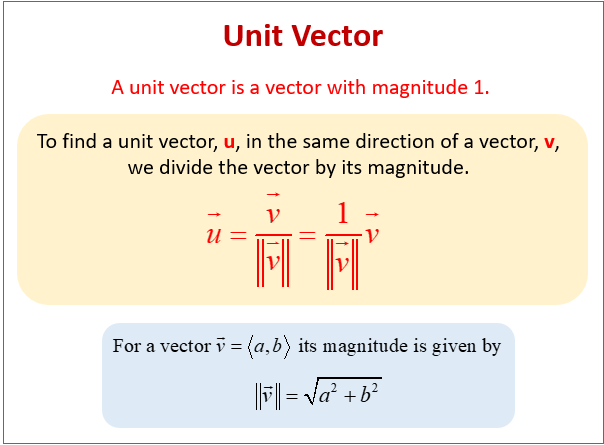
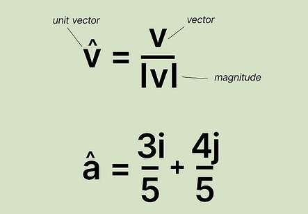
A **unit vector** is a vector whose magnitude is exactly 1 (one unit) but that still points in a particular direction. Unit vectors are useful for representing direction independently of size. They are often used to define coordinate directions (such as the x, y, and z axes) and to rewrite any vector as “magnitude × direction.”
Magnitude
The **magnitude** of a vector is the length or size of the vector. For a vector [math]\displaystyle{ \vec{v} }[/math], the magnitude is written as [math]\displaystyle{ |\vec{v}| }[/math]. Magnitude is always a non-negative scalar. In 2D and 3D, it is usually computed with the Pythagorean theorem, using the vector’s components.
Direction
The **direction** of a vector describes how it is oriented in space. It can be specified relative to axes (such as the angle from the positive x-axis), using unit vectors, or using geometric descriptions (like “30° above the horizontal” or “to the south”).
Addition and Subtraction
Vectors can be added or subtracted to form new vectors. Geometrically, we often use the **head-to-tail method** or the **parallelogram rule**. In component form, vector addition and subtraction are done by adding or subtracting corresponding components.
Scalar Multiplication
- Scalar multiplication** means multiplying a vector by a scalar (a regular number). This produces a new vector in the same or opposite direction, but with its magnitude scaled by the scalar. This is used to stretch, shrink, or reverse vectors in many physical and mathematical problems.
Dot Product
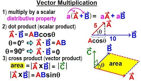
The **dot product** (or scalar product) of two vectors produces a scalar. It can be written in terms of components or in terms of magnitudes and the cosine of the angle between the vectors. Dot products are used to find angles between vectors, project one vector onto another, and calculate physical quantities such as work.
Cross Product
The **cross product** (or vector product) of two vectors in 3D produces a new vector that is perpendicular to both original vectors. Its magnitude equals the product of the magnitudes of the two vectors times the sine of the angle between them. Cross products appear in torque, angular momentum, and magnetic force, among other topics in rotational and field-based physics.
For two vectors [math]\displaystyle{ \vec{A} }[/math] and [math]\displaystyle{ \vec{B} }[/math], the magnitude of the cross product is [math]\displaystyle{ |\vec{A}\times\vec{B}| = |\vec{A}|\;|\vec{B}|\sin(\theta) }[/math], where [math]\displaystyle{ \theta }[/math] is the angle between them. The direction follows the **right-hand rule**.
Some useful properties of the cross product:
- It is **not commutative**: [math]\displaystyle{ \vec{A}\times\vec{B} \neq \vec{B}\times\vec{A} }[/math]. In fact, [math]\displaystyle{ \vec{A}\times\vec{B} = -(\vec{B}\times\vec{A}) }[/math].
- It is **distributive** over addition: [math]\displaystyle{ \vec{A}\times(\vec{B} + \vec{C}) = \vec{A}\times\vec{B} + \vec{A}\times\vec{C} }[/math].
- The cross product of a vector with itself is zero: [math]\displaystyle{ \vec{A}\times\vec{A} = \vec{0} }[/math], since the angle between a vector and itself is 0 and [math]\displaystyle{ \sin(0) = 0 }[/math].
SI Units
The **International System of Units (SI)** is the main measurement system used in science and engineering. It specifies seven base units from which all other units are built:
- meter (m) – length
- kilogram (kg) – mass
- second (s) – time
- ampere (A) – electric current
- kelvin (K) – temperature
- mole (mol) – amount of substance
- candela (cd) – luminous intensity
All physical vector quantities you encounter in this class will use combinations of these units.
Derived Units
- Derived units** are units formed by combining base units through multiplication and division. For example:
- newton (N) = kg·m/s2 (force)
- joule (J) = N·m (energy)
- watt (W) = J/s (power)
These units describe more complex physical quantities but are always traceable back to the SI base units.
Conversion
- Unit conversion** means changing a quantity from one set of units to another while representing the same physical amount. For example, converting from centimeters to meters or from kilometers per hour to meters per second. In multi-step physics problems, careful unit conversion is essential to avoid errors and to match the units expected in formulas.
Applications
Vectors and units appear in many areas:
- **Physics:** describing motion, forces, fields (electric, magnetic, gravitational), and momentum.
- **Engineering:** analyzing structures, designing mechanical systems, working with fluid flow, and modeling electrical circuits.
- **Computer Graphics:** representing positions, directions, lighting, and transformations in 2D and 3D scenes.
- **Navigation:** expressing position, velocity, and direction in GPS systems and for aircraft or ships.
Understanding how vectors and units work together lets us build accurate models and interpret real-world data correctly.
_________________________________________________________________________________________________________________________________________________________________________________________________________________________________________________________________________________________________________
What is a Vector?
In mathematics and physics, a **vector** is a quantity that has both a magnitude and a direction.
In coordinates, we often write a vector as a list of components. For example, in a 3D coordinate system, we might write: [math]\displaystyle{ \vec{v} = \langle v_x, v_y, v_z \rangle }[/math]
Here:
- [math]\displaystyle{ v_x }[/math] is the x-component of the vector,
- [math]\displaystyle{ v_y }[/math] is the y-component,
- [math]\displaystyle{ v_z }[/math] is the z-component.
A vector can also be written as a boldface letter, such as a, or with an arrow, like [math]\displaystyle{ \vec{a} }[/math]. The specific letter used often reflects the quantity: [math]\displaystyle{ \vec{v} }[/math] for velocity, [math]\displaystyle{ \vec{r} }[/math] for position, etc. Individual components of a vector are written with subscripts, such as [math]\displaystyle{ c_x }[/math] or [math]\displaystyle{ q_y }[/math].
Example of a Simple Vector
[math]\displaystyle{ \vec{v} = \langle 1, 0, 0 \rangle }[/math]
This vector has magnitude 1 and points along the positive x-direction in 3D space.
Magnitude
The **magnitude** (or length) of a vector tells us how large the vector is.
We denote the magnitude of [math]\displaystyle{ \vec{v} }[/math] using vertical bars: [math]\displaystyle{ |\vec{v}| }[/math]. You might also see notations such as [math]\displaystyle{ \overline{v} }[/math] or [math]\displaystyle{ \lVert\vec{v}\rVert_2 }[/math] (the Euclidean norm).
In a 3D system, if [math]\displaystyle{ \vec{v} = \langle v_x, v_y, v_z \rangle }[/math], then its magnitude is
[math]\displaystyle{ \lVert \vec{v} \rVert = \sqrt{v_x^2 + v_y^2 + v_z^2}. }[/math]
More generally, in n dimensions, [math]\displaystyle{ \lVert \vec{v} \rVert = \sqrt{v_1^2 + v_2^2 + \cdots + v_n^2}. }[/math]
The magnitude carries the units of the quantity being represented. For example, the magnitude of a velocity vector is speed and has units of m/s.
Note that a vector does not always represent a literal “arrow in space” between two locations. Often, a vector describes a property at a single point (like electric field at a location) or in an abstract space, even though the mathematics is the same.
Unit Vector
If we divide a nonzero vector by its magnitude, we obtain a **unit vector** in the same direction:
[math]\displaystyle{ \hat{v} = \frac{\vec{v}}{\lVert \vec{v} \rVert} }[/math].
For example, if [math]\displaystyle{ \vec{v} = \langle v_x, v_y, v_z \rangle }[/math], then
[math]\displaystyle{ \hat{v} = \frac{1}{\lVert\vec{v}\rVert}\langle v_x, v_y, v_z \rangle. }[/math]
Unit vectors are written with a “hat,” such as [math]\displaystyle{ \hat{v} }[/math]. In many coordinate systems, there are standard unit vectors. In 3D Cartesian coordinates, the unit vectors along the axes are
[math]\displaystyle{ \hat{x} = \langle 1, 0, 0 \rangle, \quad \hat{y} = \langle 0, 1, 0 \rangle, \quad \hat{z} = \langle 0, 0, 1 \rangle. }[/math]
Other coordinate systems use different unit vectors, like [math]\displaystyle{ \hat{r} }[/math] and [math]\displaystyle{ \hat{\theta} }[/math] in polar coordinates.
Direction
The **direction** of a vector tells us which way it points.
In 2D, we usually measure direction by an angle from the positive x-axis. For a vector [math]\displaystyle{ \vec{v} = \langle v_x, v_y \rangle }[/math], the direction angle [math]\displaystyle{ \theta }[/math] can be computed as
[math]\displaystyle{ \theta = \arctan\left(\frac{v_y}{v_x}\right) }[/math],
keeping track of the correct quadrant.
Simple Examples of Vector Quantities
Position
A point’s position can be written as a vector. If we have two position vectors, subtracting them gives the **relative position** from one point to the other. The magnitude of this relative position vector gives the straight-line distance between the two points. A common special case is the position relative to the origin, where the origin is at [math]\displaystyle{ \langle 0,0,0\rangle }[/math].
Velocity
- Velocity** is a vector that describes how fast and in what direction an object moves. Its magnitude is the **speed**, and it is usually measured in m/s. The velocity vector can be found by differentiating the position vector with respect to time.
For example, let [math]\displaystyle{ \vec{r}(t) = \langle t, 1, 0 \rangle\ \text{m} }[/math]. Then the velocity is
[math]\displaystyle{ \vec{v}(t) = \frac{d\vec{r}}{dt} = \langle 1, 0, 0 \rangle\ \text{m/s}. }[/math]
The speed is the magnitude of [math]\displaystyle{ \vec{v} }[/math], which in this case is 1 m/s.
Weight (Force of Gravity)
Weight is the gravitational force acting on an object; it is a vector that typically points downward. We often write the gravitational force as [math]\displaystyle{ \vec{F_g} }[/math]. In a coordinate system where +y is upward, we can write:
[math]\displaystyle{ \vec{F_g} = \langle 0, -mg, 0 \rangle, }[/math]
where [math]\displaystyle{ m }[/math] is the mass of the object and [math]\displaystyle{ g = 9.8~\text{m/s}^2 }[/math] is the magnitude of the gravitational field near Earth’s surface. The magnitude [math]\displaystyle{ |\vec{F_g}| = mg }[/math] is the weight of the object.
Visually Representing Vectors
Vectors are often drawn as **arrows**. The length of the arrow represents the magnitude, and the direction of the arrow shows which way the vector points. If a vector is tied to a particular location, the tail of the arrow is drawn at that point.
The example below shows a velocity vector for a ball moving to the right at 5 m/s.
Vector Operations
We can perform several operations on vectors, both with other vectors and with scalars. These operations are used constantly in physics and engineering. To keep the notation simple, we will describe them for 3D vectors, but they generalize naturally to higher dimensions.
Addition
For vectors [math]\displaystyle{ \vec{a} = \langle a_x, a_y, a_z \rangle }[/math] and [math]\displaystyle{ \vec{b} = \langle b_x, b_y, b_z \rangle }[/math],
[math]\displaystyle{ \vec{a} + \vec{b} = \langle a_x + b_x,\; a_y + b_y,\; a_z + b_z \rangle. }[/math]
Geometrically, we place the tail of [math]\displaystyle{ \vec{b} }[/math] at the head of [math]\displaystyle{ \vec{a} }[/math]. The vector from the tail of [math]\displaystyle{ \vec{a} }[/math] to the head of [math]\displaystyle{ \vec{b} }[/math] is the **resultant** [math]\displaystyle{ \vec{a} + \vec{b} }[/math].
Subtraction
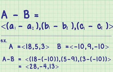
Vector subtraction can be viewed as adding the negative of a vector. We have
[math]\displaystyle{ \vec{a} - \vec{b} = \vec{a} + (-\vec{b}) = \langle a_x - b_x,\; a_y - b_y,\; a_z - b_z \rangle. }[/math]
Component-wise, we subtract each component of [math]\displaystyle{ \vec{b} }[/math] from the corresponding component of [math]\displaystyle{ \vec{a} }[/math].
Multiplication by Scalar
If [math]\displaystyle{ k }[/math] is a scalar and [math]\displaystyle{ \vec{a} = \langle a_x, a_y, a_z \rangle }[/math], then
[math]\displaystyle{ k \vec{a} = \langle k a_x,\; k a_y,\; k a_z \rangle. }[/math]
Multiplying by a positive scalar changes the magnitude but keeps the direction the same. Multiplying by a negative scalar flips the direction as well.
Division by Scalar
Dividing a vector by a nonzero scalar is equivalent to multiplying by its reciprocal:
[math]\displaystyle{ \frac{\vec{a}}{k} = \langle \frac{a_x}{k},\; \frac{a_y}{k},\; \frac{a_z}{k} \rangle. }[/math]
This operation shrinks or enlarges the vector’s magnitude while preserving (or reversing, if k is negative) its direction.
Dot Product (also called Scalar Product)
For [math]\displaystyle{ \vec{a} = \langle a_x, a_y, a_z \rangle }[/math] and [math]\displaystyle{ \vec{b} = \langle b_x, b_y, b_z \rangle }[/math], the dot product is
[math]\displaystyle{ \vec{a}\cdot\vec{b} = a_x b_x + a_y b_y + a_z b_z. }[/math]
The result is a scalar. The dot product measures how much two vectors “line up” with each other. A key property is
[math]\displaystyle{ \vec{a}\cdot\vec{b} = |\vec{a}|\;|\vec{b}|\cos(\theta), }[/math]
where [math]\displaystyle{ \theta }[/math] is the angle between [math]\displaystyle{ \vec{a} }[/math] and [math]\displaystyle{ \vec{b} }[/math]. If the dot product is zero, the vectors are perpendicular.
Cross Product (also called Vector Product)
One component-based definition of the cross product (the one often found on formula sheets) is:
[math]\displaystyle{ \vec{a} \times \vec{b} = \langle a_yb_z - a_zb_y,\; a_zb_x - a_xb_z,\; a_xb_y - a_yb_x \rangle. }[/math]
You may also see it written as
[math]\displaystyle{ \vec{a} \times \vec{b} = (a_yb_z - a_zb_y)\hat{i} - (a_zb_x - a_xb_z)\hat{j} + (a_xb_y - a_yb_x)\hat{k}. }[/math]
Although this looks complicated, the key idea is that the cross product of two 3D vectors is a new vector that is orthogonal to both of them. The order matters: changing the order flips the sign.
A common way to remember the formula is through the determinant of a 3×3 matrix:
[math]\displaystyle{ \begin{vmatrix} \hat{i} & \hat{j} & \hat{k} \\ a_x & a_y & a_z \\ b_x & b_y & b_z \end{vmatrix}. }[/math]
You can expand this determinant using cofactor expansion. Remember that the [math]\displaystyle{ \hat{j} }[/math] term has a minus sign.
You can also use online tools or videos to check your work:
- Cross product step-by-step calculator: https://www.symbolab.com/solver/vector-cross-product-calculator
- Video explanation: https://www.youtube.com/watch?v=e9T5p_Jwv5c
The magnitude of the cross product satisfies
[math]\displaystyle{ |\vec{a}\times\vec{b}| = |\vec{a}|\;|\vec{b}|\sin(\theta) }[/math],
where [math]\displaystyle{ \theta }[/math] is the angle between [math]\displaystyle{ \vec{a} }[/math] and [math]\displaystyle{ \vec{b} }[/math]. Its direction is perpendicular to the plane of [math]\displaystyle{ \vec{a} }[/math] and [math]\displaystyle{ \vec{b} }[/math] and is chosen using the Right Hand Rule. In 2D, the usual cross product is not defined.
For more mathematically-advanced students, we can connect this to linear algebra. Let [math]\displaystyle{ A \in \mathbb{R}^{m \times n} }[/math] be a matrix, and consider its **null space**:
[math]\displaystyle{ \operatorname{Null}(A) = \{ \vec{v} \in \mathbb{R}^n \mid A\vec{v} = \vec{0} \}. }[/math]
The null space is the set of all vectors that are orthogonal to every row of [math]\displaystyle{ A }[/math]. Writing the rows as [math]\displaystyle{ \vec{a}_1,\ldots,\vec{a}_m }[/math], the equation [math]\displaystyle{ A\vec{v}=\vec{0} }[/math] expands to
[math]\displaystyle{ \begin{bmatrix}\vec{a}_1 \\ \vec{a}_2 \\ \vdots \\ \vec{a}_m\end{bmatrix}\vec{v} = \begin{bmatrix}\vec{a}_1 \cdot \vec{v} \\ \vec{a}_2 \cdot \vec{v} \\ \vdots \\ \vec{a}_m \cdot \vec{v}\end{bmatrix} = \begin{bmatrix}0 \\ 0 \\ \vdots \\ 0\end{bmatrix}. }[/math]
So every vector in the null space is perpendicular to each row, and therefore to the whole row space.
For two vectors [math]\displaystyle{ \vec{a}, \vec{b} \in \mathbb{R}^3 }[/math] that are not multiples of each other, think of them as the rows of a 2×3 matrix [math]\displaystyle{ A }[/math]. The null space of [math]\displaystyle{ A }[/math] consists of all vectors orthogonal to both [math]\displaystyle{ \vec{a} }[/math] and [math]\displaystyle{ \vec{b} }[/math]. The cross product [math]\displaystyle{ \vec{a}\times\vec{b} }[/math] is (up to scaling and orientation) the unique nonzero vector in this null space once we fix the magnitude and choose a direction using the right-hand rule. This is another way to see why the cross product is perpendicular to both original vectors. In higher dimensions, the null space can have more than one dimension, so there isn’t a single unique “cross product direction” in the same way.
Another Cross Product Trick
Here is a pattern-based way to compute the cross product quickly, using components.
Suppose
[math]\displaystyle{ \vec{a} = \langle 3, -2, 4 \rangle, \quad \vec{b} = \langle -1, 6, 3 \rangle. }[/math]
We want [math]\displaystyle{ \vec{c} = \vec{a} \times \vec{b} = \langle c_x, c_y, c_z \rangle. }[/math]
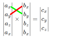
Arrange the components vertically and repeat the first component at the bottom:
[math]\displaystyle{ \begin{vmatrix} a_x \\ a_y \\ a_z \\ a_x \end{vmatrix} = \begin{vmatrix} 3 \\ -2 \\ 4 \\ 3 \end{vmatrix} }[/math], [math]\displaystyle{ \begin{vmatrix} b_x \\ b_y \\ b_z \\ b_x \end{vmatrix} = \begin{vmatrix} -1 \\ 6 \\ 3 \\ -1 \end{vmatrix} }[/math].
To find [math]\displaystyle{ c_x }[/math], draw an “X” connecting [math]\displaystyle{ a_y }[/math] with [math]\displaystyle{ b_z }[/math] and [math]\displaystyle{ a_z }[/math] with [math]\displaystyle{ b_y }[/math]:
Then compute
[math]\displaystyle{ c_x = a_y b_z - a_z b_y = (-2)(3) - (4)(6) = -6 - 24 = -30. }[/math]
For [math]\displaystyle{ c_y }[/math], use [math]\displaystyle{ a_z }[/math] with the bottom [math]\displaystyle{ b_x }[/math] and the bottom [math]\displaystyle{ a_x }[/math] with [math]\displaystyle{ b_z }[/math]:
So
[math]\displaystyle{ c_y = a_z b_x - a_x b_z = (4)(-1) - (3)(3) = -4 - 9 = -13. }[/math]
For [math]\displaystyle{ c_z }[/math], connect [math]\displaystyle{ a_x }[/math] with [math]\displaystyle{ b_y }[/math] and [math]\displaystyle{ a_y }[/math] with [math]\displaystyle{ b_x }[/math]:
Then
[math]\displaystyle{ c_z = a_x b_y - a_y b_x = (3)(6) - (-2)(-1) = 18 - 2 = 16. }[/math]
Thus
[math]\displaystyle{ \vec{a}\times\vec{b} = \langle -30, -13, 16 \rangle. }[/math]
With practice, you may not need to draw the X each time and can compute the components directly from the pattern.
Equations Involving Vector Operations
You may sometimes encounter equations that mix dot products and cross products. Two useful facts:
- [math]\displaystyle{ (\vec{w} \times \vec{v}) \cdot \vec{v} = 0 }[/math], because [math]\displaystyle{ \vec{w} \times \vec{v} }[/math] is perpendicular to both [math]\displaystyle{ \vec{w} }[/math] and [math]\displaystyle{ \vec{v} }[/math], so its dot product with either original vector is zero.
- [math]\displaystyle{ \vec{a} \cdot (\vec{b} \times \vec{c}) = (\vec{a} \times \vec{b}) \cdot \vec{c} }[/math]. This identity, called the scalar triple product identity, can be useful if one cross product is easier to compute than the other. Note that the cross product part is still order-sensitive, while the dot product is commutative.
Forms
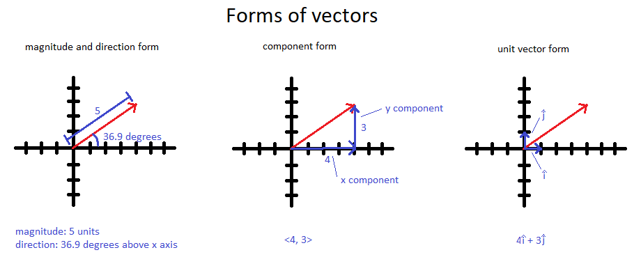
There are several common ways to describe a vector, all containing the same information.
Magnitude and Direction Form
In this form, we specify:
- The magnitude (length), and
- A description of the direction (cardinal direction, angle, or axis).
For example, “a 5 m vector at 60° above the horizontal” is in magnitude and direction form. This form is intuitive and often used in word problems and real-life descriptions.
Component Form
Here, we break the vector into components along the coordinate axes. In 3D, a vector is written as
[math]\displaystyle{ \langle a_x, a_y, a_z \rangle. }[/math]
For example, [math]\displaystyle{ \langle 2, 0, -3 \rangle }[/math] means the vector extends 2 units in +x, 0 units in y, and 3 units in -z. Most algebraic operations (like dot and cross products) are done using component form. Programming languages also typically store vectors in this way.
Unit Vector Form
In unit vector form, we write a vector as a combination of unit vectors:
[math]\displaystyle{ \hat{i} }[/math], [math]\displaystyle{ \hat{j} }[/math], [math]\displaystyle{ \hat{k} }[/math] or [math]\displaystyle{ \hat{x} }[/math], [math]\displaystyle{ \hat{y} }[/math], [math]\displaystyle{ \hat{z} }[/math].
For instance, the vector [math]\displaystyle{ \langle 2, 0, -3 \rangle }[/math] can be written as
[math]\displaystyle{ 2\hat{i} - 3\hat{k}. }[/math]
Unit vector form and component form contain the same numerical information; they just use different notation.
In n dimensions, a vector always needs n numbers to describe it fully. In 3D, magnitude–direction form uses 1 number for magnitude and 2 angles for direction, while component or unit-vector form uses 3 components.
Converting Between Forms
We can move between forms using trigonometry and the Pythagorean theorem.
- For a 2D vector [math]\displaystyle{ \vec{a} = \langle a_x, a_y \rangle }[/math], the magnitude is
[math]\displaystyle{ |\vec{a}| = \sqrt{a_x^2 + a_y^2}. }[/math]
- The direction angle from the positive x-axis is
[math]\displaystyle{ \theta = \tan^{-1}\left(\frac{a_y}{a_x}\right) }[/math] (with quadrant checks).
- Given magnitude [math]\displaystyle{ |\vec{a}| }[/math] and angle [math]\displaystyle{ \theta }[/math], the components are
 [math]\displaystyle{ a_x = |\vec{a}|\cos\theta }[/math],
 [math]\displaystyle{ a_y = |\vec{a}|\sin\theta }[/math].
Vectors in VPython
In VPython (used in GlowScript), vectors are represented by the type vec or vector. The constructor takes three arguments: the x, y, and z components.
Example:
velocity = vec(3, -1, 2)
This creates a vector called velocity with components (3, -1, 2).
In VPython’s default view, +x points to the right, +y points upward, and +z points out of the screen toward the viewer.
Modifying Vectors
You can access or modify individual components using .x, .y, and .z. For example:
velocity.x = 5
changes the x-component from 3 to 5.
Helpful Vector Functions
Magnitude
VPython provides the mag function to compute the magnitude of a vector:
velocity = vec(3, -1, 2)
speed = mag(velocity)  # magnitude of velocity
Normalize
To obtain a unit vector in the same direction (normalize a vector), use norm:
v = vec(5, 0, 0)
v_hat = norm(v)  # v_hat = <1, 0, 0>
Dot and Cross Product
The functions dot and cross compute dot and cross products:
a = vec(1, 2, 3)
b = vec(4, 5, 6)
dot_prod = dot(a, b)      # a · b
cross_prod = cross(a, b)  # a × b
Visualization
To visualize vectors, VPython provides the arrow object. You specify:
pos– tail position,axis– direction and length of the arrow (a vector).
Optional parameters include shaftwidth, headwidth, and headlength. You can also change attributes like color. See more details here.
Example of a velocity vector arrow at the origin:
velocity = vec(1, 1, 0)
origin = vec(0, 0, 0)
shaftwidth = 0.1
vel_arrow = arrow(pos=origin, axis=velocity,
shaftwidth=shaftwidth, color=color.red)
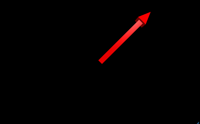 Output in VPython of Visualized Vector
A Computational Model
Click here to run the interactive computational model.
This model walks through basic vector operations step by step. It starts by defining vectors as arrows, then explores:
- Addition and subtraction
- Scalar multiplication
- Magnitude and unit vectors
- Dot and cross products
Each operation is shown both in formula form and using VPython shortcut functions. You can edit the vector values and rerun the code to see how the results change. Commenting out parts of the script can help you focus on one type of operation at a time.
Examples
Very Simple
Vector [math]\displaystyle{ \vec{a} = \langle 2.5, 7.4, 8.0 \rangle }[/math]. Find its magnitude and a unit vector in its direction.
- Solution:**
First, find the magnitude:
[math]\displaystyle{ |\vec{a}| = \sqrt{2.5^2 + 7.4^2 + 8.0^2} }[/math]
[math]\displaystyle{ = \sqrt{6.25 + 54.76 + 64} }[/math]
[math]\displaystyle{ = \sqrt{125.01} \approx 11.18. }[/math]
Now form the unit vector:
[math]\displaystyle{ \hat{a} = \frac{\vec{a}}{|\vec{a}|} = \left\langle \frac{2.5}{11.18}, \frac{7.4}{11.18}, \frac{8.0}{11.18} \right\rangle \approx \langle 0.224, 0.662, 0.716 \rangle. }[/math]
So the magnitude is about 11.18, and the direction can be described by the unit vector [math]\displaystyle{ \langle 0.224, 0.662, 0.716 \rangle }[/math].
Simple
Let [math]\displaystyle{ \vec{a} = \langle 2, 4, 2 \rangle }[/math] and [math]\displaystyle{ \vec{b} = \langle -1, 1, 3 \rangle }[/math]. Find the magnitude of [math]\displaystyle{ \vec{a} - 2\vec{b} }[/math].
- Solution:**
Compute the combination:
[math]\displaystyle{ \vec{a} - 2\vec{b} = \langle 2, 4, 2 \rangle - 2\langle -1, 1, 3 \rangle }[/math]
[math]\displaystyle{ = \langle 2, 4, 2 \rangle - \langle -2, 2, 6 \rangle }[/math]
[math]\displaystyle{ = \langle 4, 2, -4 \rangle. }[/math]
Now find the magnitude:
[math]\displaystyle{ |\langle 4, 2, -4 \rangle| = \sqrt{4^2 + 2^2 + (-4)^2} = \sqrt{16 + 4 + 16} = \sqrt{36} = 6. }[/math]
Intermediate
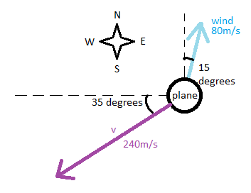
An airplane is flying in still air at 240 m/s, 35° south of west. A wind blows at 80 m/s, 15° east of north. What must the plane’s new velocity relative to the air be in order to keep the same overall trajectory? Give your answer in components (with +x east and +y north).
- Solution:**
Let
- [math]\displaystyle{ \vec{v_{p,0}} }[/math] = original velocity of the plane (relative to air),
- [math]\displaystyle{ \vec{v_w} }[/math] = wind velocity (relative to ground),
- [math]\displaystyle{ \vec{v_{p,1}} }[/math] = new plane velocity (relative to air).
We want the **resultant ground velocity** of the plane to stay equal to [math]\displaystyle{ \vec{v_{p,0}} }[/math]. The velocity relative to the ground is
[math]\displaystyle{ \vec{v_{p,1}} + \vec{v_w}. }[/math]
So we require
[math]\displaystyle{ \vec{v_{p,1}} + \vec{v_w} = \vec{v_{p,0}} }[/math] [math]\displaystyle{ \Rightarrow \vec{v_{p,1}} = \vec{v_{p,0}} - \vec{v_w}. }[/math]
Express everything in components:
Take +x as east and +y as north.
35° south of west corresponds to 215° from the +x-axis:
[math]\displaystyle{ \vec{v_{p,0}} = \langle 240\cos(215^\circ),\; 240\sin(215^\circ) \rangle \approx \langle -196.6,\; -137.7 \rangle\ \text{m/s}. }[/math]
15° east of north corresponds to 75° from the +x-axis:
[math]\displaystyle{ \vec{v_w} = \langle 80\cos(75^\circ),\; 80\sin(75^\circ) \rangle \approx \langle 20.7,\; 77.3 \rangle\ \text{m/s}. }[/math]
Now subtract:
[math]\displaystyle{ \vec{v_{p,1}} = \vec{v_{p,0}} - \vec{v_w} = \langle -196.6, -137.7 \rangle - \langle 20.7, 77.3 \rangle }[/math]
[math]\displaystyle{ = \langle -217.3,\; -214.9 \rangle\ \text{m/s}. }[/math]
So the plane must adjust its airspeed to approximately [math]\displaystyle{ \langle -217.3,\; -214.9 \rangle }[/math] m/s relative to the air to keep its original track.
Difficult
Find the angle between the vectors [math]\displaystyle{ \langle 2, 5, -2 \rangle }[/math] and [math]\displaystyle{ \langle 3, -4, -1 \rangle }[/math].
- Solution:**
Use the dot product formula:
[math]\displaystyle{ \vec{a}\cdot\vec{b} = |\vec{a}|\;|\vec{b}|\cos\theta. }[/math]
So
[math]\displaystyle{ \theta = \cos^{-1}\left(\frac{\vec{a}\cdot\vec{b}}{|\vec{a}|\;|\vec{b}|}\right). }[/math]
Compute the numerator:
[math]\displaystyle{ \vec{a}\cdot\vec{b} = 2(3) + 5(-4) + (-2)(-1) = 6 - 20 + 2 = -12. }[/math]
Compute the magnitudes:
[math]\displaystyle{ |\vec{a}| = \sqrt{2^2 + 5^2 + (-2)^2} = \sqrt{4 + 25 + 4} = \sqrt{33}, }[/math]
[math]\displaystyle{ |\vec{b}| = \sqrt{3^2 + (-4)^2 + (-1)^2} = \sqrt{9 + 16 + 1} = \sqrt{26}. }[/math]
So
[math]\displaystyle{ \theta = \cos^{-1}\left(\frac{-12}{\sqrt{33}\sqrt{26}}\right) = \cos^{-1}\left(\frac{-12}{\sqrt{858}}\right) \approx 114^\circ. }[/math]
Connectedness
Vectors appear in many everyday and engineering contexts.
Consider a desk. Its weight is a force vector pointing downward, the normal force from the floor is a vector pointing upward, and the forces among the desk’s parts can all be represented as vectors. Measurements such as the diagonal distance across the desktop can also be seen as vectors from one corner to another.
Your motion can be described using vectors as well. Your **position** relative to some reference point can be written as a position vector. The difference between two position vectors is a displacement vector. **Velocity** describes how your position changes over time; it is the time derivative of the position vector, and its magnitude is your speed. **Acceleration** is the time derivative of velocity. All of these quantities can be broken into components, which makes it easier to analyze motion in each direction separately.
In Physics 2 and beyond, vectors are everywhere. The electric field, magnetic field, many forces, and other quantities are all vector fields. For example, the magnetic force on a charged particle is
[math]\displaystyle{ \vec{F} = q\;\vec{v} \times \vec{B}, }[/math]
which combines a cross product of two vectors and a scalar multiplication.
Even outside physics, vectors are central. In engineering, they are used for stress analysis, fluid flow, and control systems. In computer science, vectors appear in graphics, simulations, robotics, and machine learning (where data points are often vectors in high-dimensional spaces). Virtually any physical or abstract quantity that has both “how much” and “which way” can be modeled as a vector.
History
Ideas similar to vectors go back many centuries. Early uses treated them as directed line segments rather than abstract quantities. Hero of Alexandria’s work Mechanics in the first century AD contains one of the earliest known discussions of adding such directed segments.
In the 18th and 19th centuries, several mathematicians used 2D vectors to represent complex numbers. Caspar Wessel, Jean-Robert Argand, Carl Friedrich Gauss, and William Rowan Hamilton all contributed to this viewpoint. One component represented the real part, and the other represented the imaginary part. Hamilton also introduced the term “vector.”
August Ferdinand Möbius, in his 1827 book The Barycentric Calculus, formalized many vector ideas, including labeling vectors with letters and defining scalar multiplication. Hermann Grassmann, in his 1844 work Ausdehnungslehre (“The Calculus of Extension”), developed a more general theory of vectors in spaces of arbitrary dimension and laid foundations for linear algebra.
The modern vector notation and conventions used in physics owe a lot to J. Willard Gibbs and Oliver Heaviside in the late 19th century. They refined vector methods and used them to express Maxwell’s equations of electromagnetism in the compact form we study today.
See Also
External Links
Mathematical computations on vectors (MIT OCW notes): http://ocw.mit.edu/courses/mathematics/18-02sc-multivariable-calculus-fall-2010/1.-vectors-and-matrices/part-a-vectors-determinants-and-planes/session-1-vectors/MIT18_02SC_notes_0.pdf
Computational work with vectors in VPython: http://vpython.org/contents/docs/vector.html
Basic vector introduction: https://www.physics.uoguelph.ca/tutorials/vectors/vectors.html
Further Reading
- *Vector Analysis* – Josiah Willard Gibbs
- *Introduction to Matrices and Vectors* – Jacob T. Schwartz
References
https://mathinsight.org/definition/magnitude_vector https://www.mathsisfun.com/algebra/vectors.html http://ocw.mit.edu/courses/mathematics/18-02sc-multivariable-calculus-fall-2010/1.-vectors-and-matrices/part-a-vectors-determinants-and-planes/session-1-vectors/MIT18_02SC_notes_0.pdf http://mathinsight.org/vector_introduction http://www.math.mcgill.ca/labute/courses/133f03/VectorHistory.html https://www.glowscript.org/docs/VPythonDocs/vector.html https://www.glowscript.org/docs/VPythonDocs/arrow.html https://www.britannica.com/science/vector-mathematics https://www.grc.nasa.gov/www/k-12/rocket/vectcomp.html https://www.onlinemathlearning.com/dot-product.html
