VPython Animation

This page is established to aid students in understanding how their coding in VPython affects the animation, and how they can make changes to their codes to reflect what they want in VPython.

The Basic Concept Behind VPython Animation

What greatly differs VPython from ordinary Python is that through IDLE, the interactive development environment, and the use of "visual," one can animate any 3D object in real time. The key aspect to using animation in VPython is within the first two lines of starting code:

from __future__ import division
from visual import*

Uses of Animation

Through VPython animation, one can accomplish various goals. Whether it's modeling a 3D structure to observe how it would react in the real world under specific circumstances, or modeling concepts that are too small to see or reactions not visible to the naked eye - such as the reaction between 2 wires or a ball in a magnetic field.

Methods to Changing Your Animation

Loops

The most effective way to change your animation is through loops. Arrows, balls, squares, and other objects are all subject to animation within VPython. The easiest way to do so - updating the position within the while loop. By updating variables in loops - the position, direction, speed, acceleration, and many other variables can be updated - one can cause the appearance of movement.

By updating the position of the object, the animation begins. However, in order to update position to a more accurate degree, the position must account for any forces acting on the object - such as gravity, magnetic fields, friction, etc.

The following code is a section taken from PHYS 2212 Lab 6 where animation occurs

while proton.x<5e-10:
rate(100)

r1=barrow1.pos-proton.pos
rmag1=mag(r1)
rhat1 = r1/rmag1

r2=barrow2.pos-proton.pos
rmag2=mag(r2)
rhat2 = r2/rmag2

r3=barrow3.pos-proton.pos
rmag3=mag(r3)
rhat3 = r3/rmag3

r4=barrow4.pos-proton.pos
rmag4=mag(r4)
rhat4 = r4/rmag4

B1=C*cross(velocity,rhat1)*q/(rmag1**2)
B2=C*cross(velocity,rhat2)*q/(rmag2**2)
B3=C*cross(velocity,rhat3)*q/(rmag3**2)
B4=C*cross(velocity,rhat4)*q/(rmag4**2)

barrow1.axis = B1*scalefactor
barrow2.axis = B2*scalefactor
barrow3.axis = B3*scalefactor
barrow4.axis = B4*scalefactor
proton.pos = proton.pos+velocity*deltat

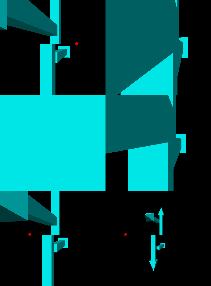
Animation of antiproton in a Magnetic Field

Changing Rate

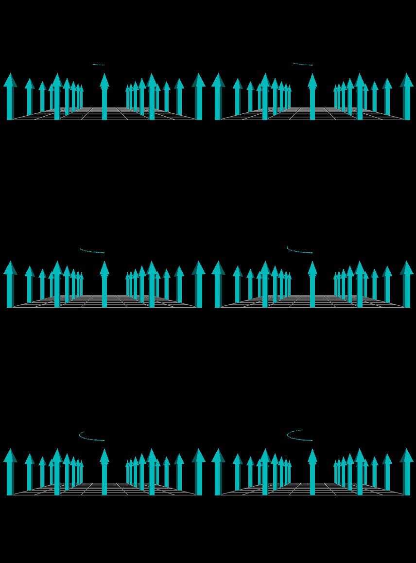
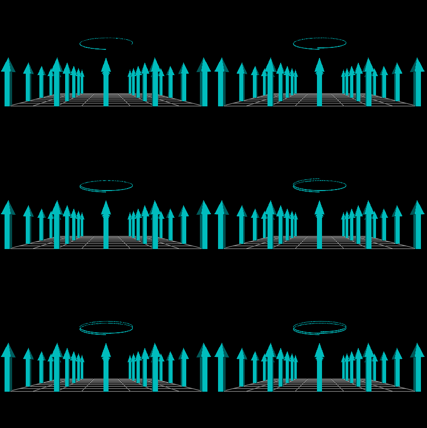
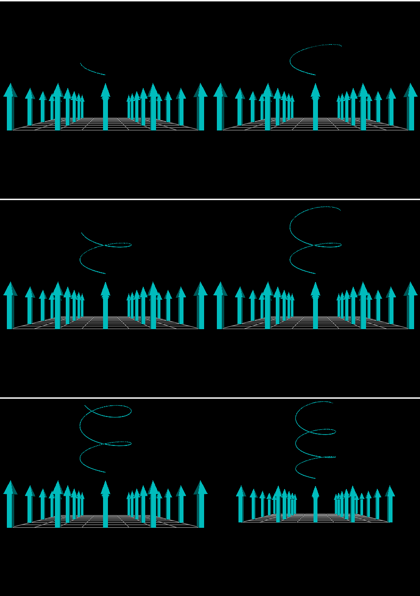
Within any loop, one may establish a rate. This rate serves as the speed at which the animation is performed within VPython. The rate value indicates that the computer will calculate X times in one second. By increasing the rate, the animation appears to move faster. On the other hand, decreasing the rate makes the animation appear to move much slower. Sometimes, by changing the rate, you can look for specific reactions or movements in the animation.

Example

A particle moving through a magnetic field, taken from PHYS 2212 - Lab 9 Magnetic Force. By updating the rate, the animation can appear to be faster - while other aspects like the max time or updating velocity and position serve to move the ball within the magnetic field.

from __future__ import division
from visual import *

B0 = vector(0,0.2,0)

xmax = .4
dx = .1
yg = -.1

for x in arange(-xmax, xmax+dx, dx):
curve(pos=[(x,yg,-xmax),(x,yg,xmax)], color=(.7,.7,.7))
for z in arange(-xmax, xmax+dx, dx):
curve(pos=[(-xmax,yg,z),(xmax,yg,z)],color=(.7,.7,.7))
bscale = 1
for x in arange(-xmax, xmax+dx, 2*dx):
for z in arange(-xmax, xmax+dx, 2*dx):
arrow(pos=(x,yg,z), axis=B0*bscale, color=(0,.8,.8))

deltat = 1e-11
t = 0
particle = sphere(pos = vector(0,.15,.3), radius = 1e-6, color=color.cyan)
velocity = vector(-2e6,2e4,0)
q = -1.6e-19
mass = 1.7e-27
p = mass*velocity
trail = curve(color = particle.color)
while t<1.67e-6:
rate(3000)
x = q*velocity
Fb = cross(x,B0)
p = p + Fb*deltat
velocity = p/mass
particle.pos = particle.pos + velocity*deltat
trail.append(pos=particle.pos)
if particle.pos.x == 0:
print (t)
t=t+deltat

Rate at (400)

Rate at (4000)

Rate at (4000), Increased Y velocity

Connectedness

How is this topic connected to something that you are interested in?

VPython itself is a very interesting language to work with coding wise. I originally learned coding through Java, and become more proficient through Matlab. Having done an animation project in Matlab, I was already intrigued by the different ways you can code something to perform to your desires. However, in Matlab, animation wasn't always the easiest goal to achieve. Thus, when we started using VPython, and the animation was very straight-forward and smooth, I immediately enjoyed experimenting with it.

How is it connected to your major?

I myself am a Materials Science and Engineering major, so there isn't much coding to be seen. However, if you are trying to see how a material will fail or the way it acts in certain situations, VPython is a good method to model what you are doing in 3D and to be actually be able to visualize your material.

Is there an interesting industrial application?

An interesting industrial application is the 3D modeling aspect. While yes, there are more advanced programs to aid in 3D modeling, VPython works as a basic understanding and would be more useful in classroom settings (such as PHYS 2211/2212) and for basic demonstrations.

History

Ever since VPython was first established animation has been a key aspect. However, over the past few decades, improvements have been made - ranging from higher efficiency through "shortcuts" and new commands to new objects and bug fixes. Over time, VPython has become easier to use and is seen more within schools and classes as a great learning program.

References

https://www.youtube.com/watch?v=cNdPqgNFeVk http://vpython.org/contents/docs/