VPython Modelling of Electric and Magnetic Forces: Difference between revisions
(I have expanded on the specifics of mathematical and computational models of electric and magnetic forces. I made a VPython example for electric forces, and I also commented on the VPython code to show what each step actually does. Connectedness) |
|||
| (40 intermediate revisions by 2 users not shown) | |||
| Line 1: | Line 1: | ||
VPython Modeling of Electric and Magnetic Forces | VPython Modeling of Electric and Magnetic Forces | ||
Claimed By: Griffin Bonnett Spring 2017 | |||
Claimed By: Griffin Bonnett Spring 2017 4/09/2017 | |||
Claimed by: Yunqing Jia Fall 2017 | |||
==The Main Idea== | ==The Main Idea== | ||
Vpython is a programming language designed to model physics properties in a 3D simulation. This section we will be focused on modeling the electric and magnetic forces in Vpython. | Vpython is a programming language designed to model physics properties in a 3D simulation. It consists of the Python programming languange with an additional module called Visual that creates the environment to generate models in 3D. This section we will be focused on modeling the electric and magnetic forces in Vpython. | ||
===A Mathematical Model=== | ===A Mathematical Model=== | ||
When you | |||
When you are starting a new Vpython program, first write out all the equations and constants you might need, and then define the variables in their appropriate forms such as vectors, arrows, or spheres. | |||
:''Electric Force'' | |||
::<math>\vec F={q}_{2}\times\vec{E}_{1} </math> | |||
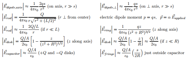
::equations for electric fields(vec{E}) | |||
::[[File:equationsForElectricFields.PNG]] | |||
::[http://www.physicsbook.gatech.edu/Electric_Force derivation] | |||
:''Magnetic Force'' | |||
::<math>{\vec{F} = q\vec{v}\times\vec{B}}</math> | |||
::equations for magnetic fields(vec{B}) | |||
::[[File:equationsForMagneticFields.PNG]] | |||
::[http://www.physicsbook.gatech.edu/Magnetic_Force derivation] | |||
The equations are the mathematical basis for computational simulations. After defining constants and initializing variables in the initial state, you can now mathematically update the position, electric/magnetic field, electric/magnetic force in the next small time step. In order to show this at different times and/or locations, you can simply iterate the same process with the new values. Since it is an iterated process, VPython can only give us an approximate model. To display time-varying electric or magnetic field, one can decrease the time increment in each step to make the approximation more accurate. | |||
===A Computational Model=== | ===A Computational Model=== | ||
This is when we begin to program using Vpython. A finished and working program will give us the ability to visualize the physics of magnetic and electric forces. Vpython can be used to model any number of other physical interactions as well such as springs and gravity. Running a simulation allows us to view concepts that would not be observable any other way especially on the same | This is when we begin to program using Vpython. | ||
1. Initialize constants | |||
2. Set initial conditions | |||
3. Write a loop | |||
:''in the loop, you will (not all steps are included depending on the problem)'' | |||
::i. update electric / magnetic fields if they are time-variant | |||
::ii. update electric / magnetic forces | |||
::iii. update momentum / velocity if the observed target is a moving object | |||
::iv. update particle position | |||
A finished and working program will give us the ability to visualize the physics of magnetic and electric forces. Vpython can be used to model any number of other physical interactions as well such as springs and gravity. Running a simulation allows us to view concepts that would not be observable any other way especially on the same timescale. We are able to visibly observe magnetic and electric fields in a dynamic situation which is difficult to visualize without a model. This also allows for many more calculations to be performed and the ability to interpolate and extrapolate data. | |||
==Examples== | ==Examples== | ||
===Electric Force Model=== | |||
[http://www.glowscript.org/#/user/JJ129816/folder/Private/program/electricForce ElectricForceModel] | |||
===Magnetic Force Model=== | ===Magnetic Force Model=== | ||
[http://www.glowscript.org/#/user/griffinbonnett/folder/Public/program/vPython MagForceModel] | |||
[[File:MagForcePic.JPG]] | |||
For Magnetic forces: | For Magnetic forces: | ||
| Line 25: | Line 67: | ||
field. | field. | ||
''Step 1: Frame the problem in fundamental ideas or equations'' | '''Step 1: Frame the problem in fundamental ideas or equations''' | ||
This is where you write down anything the problem gives you. | This is where you write down anything the problem gives you. | ||
Equations: Constants: | '''Equations:''' '''Constants:''' | ||
F = q·v x B Charge of the particle(q) | F = q·v x B Charge of the particle(q) | ||
dp/dt = Fnet Velocity vector of the particle(v) | dp/dt = Fnet Velocity vector of the particle(v) | ||
| Line 39: | Line 81: | ||
Due to our understanding of how magnetic fields cause a force on a moving charged particle, we can craft a general outline for the calculations. We can also find expected values and predict the behavior of the model. We will need to calculate the magnetic force and use it to update its position and velocity. | Due to our understanding of how magnetic fields cause a force on a moving charged particle, we can craft a general outline for the calculations. We can also find expected values and predict the behavior of the model. We will need to calculate the magnetic force and use it to update its position and velocity. | ||
| Line 50: | Line 90: | ||
'''Initialize the variables''' | '''Initialize the variables''' | ||
B0 = vector(0,1,0) ''#initial magnetic field'' | |||
particle = sphere(pos=(0, | particle = sphere(pos=(0, 0,.3), radius = .01, color = color.red) ''#create particle and set initial position'' | ||
velocity = vector( | velocity = vector(2e6,1e6,0) ''#initial velocity'' | ||
q = | q = 1.6e-19 ''#constant: Coulombs of charge in one particle'' | ||
m = 1.7e-27 | m = 1.7e-27 ''#constant: mass of particle'' | ||
trail = curve(color=particle.color) | trail = curve(color=particle.color) ''#establish visualization of the force'' | ||
deltat = 1e-11 | deltat = 1e-11 ''#time increments'' | ||
t = 0 | t = 0 ''#initial time'' | ||
'''The Loop''' | '''The Loop''' | ||
while t < 1. | |||
while t < 1.3e-3: | |||
rate(10000) | rate(10000) | ||
## Insert the necessary steps inside the loop below to update the particle's position and velocity | ## Insert the necessary steps inside the loop below to update the particle's position and velocity | ||
## a) | ## a)calculate the needed quantities to update the particle's velocity | ||
p = m * velocity | p = m * velocity | ||
Fnet= q * cross(velocity, B0) | Fnet= q * cross(velocity, B0) | ||
p = p + Fnet*deltat | p = p + Fnet*deltat | ||
## b) | ## b)update the particle's velocity | ||
velocity = p/m | velocity = p/m | ||
## c) Update the position of the proton (movies in a straight line initially). | ## c) Update the position of the proton (movies in a straight line initially). | ||
particle.pos = particle.pos + velocity*deltat | particle.pos = particle.pos + velocity*deltat | ||
| Line 75: | Line 117: | ||
t=t+deltat | t=t+deltat | ||
The method used to simulate magnetic force would work equally well to simulate the electric force. | |||
==Connectedness== | ==Connectedness== | ||
#How is this topic connected to something that you are interested in? | #How is this topic connected to something that you are interested in? | ||
::I am fascinated by 3D modeling. I have begun to teach my self Blender recently. Even though there is less programming involved, Blender incorporates much of the fundamentals that VPython uses such as vector math and using iterations of functions to achieve the desired output. I believe that computational models are great learning aids for people to visualize concepts in 3D, such as electric and magnetic fields and forces, especially when the path becomes complex and more mathematical iterations are required. | |||
#How is it connected to your major? | #How is it connected to your major? | ||
::VPython, electric and magnetic forces, and simulations are fundamental to my major as an electrical engineer. I can use Vpython to simulate how certain electrical components that would interact with a magnetic field. I could also use it to simulate the electromagnetic interactions at the quantum level. | |||
#Is there an interesting industrial application? | #Is there an interesting industrial application? | ||
::Industry routinely uses VPython to simulate optimal efficiency. This can give a baseline to test the efficiency of industrial machines or processes. These simulations can help identify ways to improve the bottom line of a company. The simulations can also save money in research and development by replacing some more costly experimental testing. | |||
==History== | ==History== | ||
The cT programming language was created in 1985 by researchers at Carnegie Mellon University. Even though it had other applications, it was mainly a 2d graphics learning tool. | |||
As David Scherer began college in 1998, he was being taught physics using cT. Scherer saw some flaws in cT and set out to improve it. By 2000,Scherer, with help from David Andersen, Ruth Chabay, Ari Heitner, Ian Peters, and Bruce Sherwood, created Visual, a module for Python that was easier than cT and could render in 3D. The name VPython comes from merging Visual and Python together. The development of VPython made cT obsolete and Vpython took its place. | |||
The most recent change in the VPython is the developers announced in 2016 that they will no longer be producing the classic software. Instead, the will focus on implementing the programming language in Glowscript and Jupyter. | |||
== See also == | == See also == | ||
| Line 98: | Line 148: | ||
Internet resources on this topic | Internet resources on this topic | ||
http://www.glowscript.org/#/user/GlowScriptDemos/folder/matterandinteractions/program/MatterAndInteractions | |||
https://trinket.io/welcome | |||
https://www.revolvy.com/main/index.php?s=VPython&item_type=topic | |||
==References== | ==References== | ||
| Line 104: | Line 162: | ||
[[Category:Which Category did you place this in?]] | [[Category:Which Category did you place this in?]] | ||
https://www.revolvy.com/main/index.php?s=VPython&item_type=topic | |||
http://www.glowscript.org/#/user/griffinbonnett/folder/Public/program/vPython | |||
Latest revision as of 00:42, 30 November 2017
VPython Modeling of Electric and Magnetic Forces
Claimed By: Griffin Bonnett Spring 2017 4/09/2017
Claimed by: Yunqing Jia Fall 2017
The Main Idea
Vpython is a programming language designed to model physics properties in a 3D simulation. It consists of the Python programming languange with an additional module called Visual that creates the environment to generate models in 3D. This section we will be focused on modeling the electric and magnetic forces in Vpython.
A Mathematical Model
When you are starting a new Vpython program, first write out all the equations and constants you might need, and then define the variables in their appropriate forms such as vectors, arrows, or spheres.
- Electric Force
- [math]\displaystyle{ \vec F={q}_{2}\times\vec{E}_{1} }[/math]
- equations for electric fields(vec{E})
- derivation

- Magnetic Force
- [math]\displaystyle{ {\vec{F} = q\vec{v}\times\vec{B}} }[/math]
- equations for magnetic fields(vec{B})

- derivation

The equations are the mathematical basis for computational simulations. After defining constants and initializing variables in the initial state, you can now mathematically update the position, electric/magnetic field, electric/magnetic force in the next small time step. In order to show this at different times and/or locations, you can simply iterate the same process with the new values. Since it is an iterated process, VPython can only give us an approximate model. To display time-varying electric or magnetic field, one can decrease the time increment in each step to make the approximation more accurate.
A Computational Model
This is when we begin to program using Vpython.
1. Initialize constants
2. Set initial conditions
3. Write a loop
- in the loop, you will (not all steps are included depending on the problem)
- i. update electric / magnetic fields if they are time-variant
- ii. update electric / magnetic forces
- iii. update momentum / velocity if the observed target is a moving object
- iv. update particle position
A finished and working program will give us the ability to visualize the physics of magnetic and electric forces. Vpython can be used to model any number of other physical interactions as well such as springs and gravity. Running a simulation allows us to view concepts that would not be observable any other way especially on the same timescale. We are able to visibly observe magnetic and electric fields in a dynamic situation which is difficult to visualize without a model. This also allows for many more calculations to be performed and the ability to interpolate and extrapolate data.
Examples
Electric Force Model
Magnetic Force Model

For Magnetic forces: We are going to simulate the motion of a charged particle immersed in a magnetic field.
Step 1: Frame the problem in fundamental ideas or equations
This is where you write down anything the problem gives you.
Equations:           Constants:
F = q·v x B          Charge of the particle(q)
dp/dt = Fnet         Velocity vector of the particle(v)
p = ma               Magnetic field vector(B)
v= p/m               Mass of particle (m)
Due to our understanding of how magnetic fields cause a force on a moving charged particle, we can craft a general outline for the calculations. We can also find expected values and predict the behavior of the model. We will need to calculate the magnetic force and use it to update its position and velocity.
Step2: Conceptualize the problem
We want to show the particle moving through space relative to time. Since computer programs only comprehend discreet values, we will want to move through time in discreet increments. We do this by using a while loop because while t is less than a certain value the loop will continue to be updated. We can put the limit of t to anytime so long as the rate is high enough to run the program reasonably fast and t is large enough to run the full length simulation. We will set the initial time to t = 0 and add a constant delta t to each iteration in the while loop. Each new iteration of time will allow us to update the position and velocity vector. To update these values, conservation of momentum is used to relate the magnetic and the position and velocity.
   Initialize the variables
    B0 = vector(0,1,0)  #initial magnetic field
    particle = sphere(pos=(0, 0,.3), radius = .01, color = color.red)  #create particle and set initial position
    velocity = vector(2e6,1e6,0)  #initial velocity
    q = 1.6e-19  #constant: Coulombs of charge in one particle
    m = 1.7e-27  #constant: mass of particle
    trail = curve(color=particle.color)  #establish visualization of the force
    deltat = 1e-11  #time increments
    t = 0  #initial time
   The Loop

   while t < 1.3e-3:
   rate(10000)
   ## Insert the necessary steps inside the loop below to update the particle's position and velocity
   ## a)calculate the needed quantities to update the particle's velocity
   p = m * velocity
   Fnet= q * cross(velocity, B0)
   p = p + Fnet*deltat

   ## b)update the particle's velocity
   velocity = p/m

   ## c) Update the position of the proton (movies in a straight line initially).
   particle.pos = particle.pos + velocity*deltat
   trail.append(pos=particle.pos)
   t=t+deltat
The method used to simulate magnetic force would work equally well to simulate the electric force.
Connectedness
- How is this topic connected to something that you are interested in?
- I am fascinated by 3D modeling. I have begun to teach my self Blender recently. Even though there is less programming involved, Blender incorporates much of the fundamentals that VPython uses such as vector math and using iterations of functions to achieve the desired output. I believe that computational models are great learning aids for people to visualize concepts in 3D, such as electric and magnetic fields and forces, especially when the path becomes complex and more mathematical iterations are required.
- How is it connected to your major?
- VPython, electric and magnetic forces, and simulations are fundamental to my major as an electrical engineer. I can use Vpython to simulate how certain electrical components that would interact with a magnetic field. I could also use it to simulate the electromagnetic interactions at the quantum level.
- Is there an interesting industrial application?
- Industry routinely uses VPython to simulate optimal efficiency. This can give a baseline to test the efficiency of industrial machines or processes. These simulations can help identify ways to improve the bottom line of a company. The simulations can also save money in research and development by replacing some more costly experimental testing.
History
The cT programming language was created in 1985 by researchers at Carnegie Mellon University. Even though it had other applications, it was mainly a 2d graphics learning tool.
As David Scherer began college in 1998, he was being taught physics using cT. Scherer saw some flaws in cT and set out to improve it. By 2000,Scherer, with help from David Andersen, Ruth Chabay, Ari Heitner, Ian Peters, and Bruce Sherwood, created Visual, a module for Python that was easier than cT and could render in 3D. The name VPython comes from merging Visual and Python together. The development of VPython made cT obsolete and Vpython took its place.
The most recent change in the VPython is the developers announced in 2016 that they will no longer be producing the classic software. Instead, the will focus on implementing the programming language in Glowscript and Jupyter.
See also
Are there related topics or categories in this wiki resource for the curious reader to explore? How does this topic fit into that context?
Further reading
Books, Articles or other print media on this topic
External links
Internet resources on this topic
https://www.revolvy.com/main/index.php?s=VPython&item_type=topic
References
This section contains the the references you used while writing this page
https://www.revolvy.com/main/index.php?s=VPython&item_type=topic
http://www.glowscript.org/#/user/griffinbonnett/folder/Public/program/vPython