Vectors
This page defines and describes vectors.
The Main Idea
In mathematics and physics, a vector is a quantity with both a magnitude and a direction in space. The magnitude of a vector is a scalar value which can represent a variety of characteristics, depending on the situation. The magnitude of the vector (and the vector itself) has units corresponding to the characteristic it represents. The direction of a vector is simply an orientation in space giving context to the magnitude.
Simple examples of vector quantities
To understand what it means for a vector to have both a magnitude and a direction, and to understand why the magnitude and direction together are often considered a single quantity, it can be helpful to consider an example. The Velocity of an object is an example of a vector quantity. The speed of the object, often given in meters per second (m/s), is a scalar value describing how quickly the object is moving. Speed is the magnitude of the velocity vector. However, the object's movement happens in a particular spatial direction, which the speed alone does not tell us. The direction of the object's movement is also a part of the velocity vector. Together, speed and direction comprise the velocity vector and give a complete description of an object's motion at a point in time. Another example of a vector is position; the distance of a point from the origin of a coordinate system can be represented as the magnitude of a vector, and this distance together with a direction describes exactly where a point can be found.
Notation
A variable representing a vector is typically written as a letter with an arrow over it: [math]\displaystyle{ \vec{a} }[/math]. The arrow may one-sided to make it easier to write. Alternatively, a vector variable might simply be written as a boldface letter: a. Which letter is used depends on the context; for example, [math]\displaystyle{ \vec{v} }[/math] represents velocity.
Surrounding a vector by | symbols denotes its magnitude: [math]\displaystyle{ |\vec{b}| }[/math].
A unit vector is a vector whose magnitude is 1 by design. A unit vector is denoted by a letter with a ^ symbol (called a "hat") written over it: [math]\displaystyle{ \hat{c} }[/math] (read as "c-hat").
Some unit vectors are normalized regular vectors. For example, [math]\displaystyle{ \hat{a} }[/math] is the normalized version of the vector [math]\displaystyle{ \vec{a} }[/math]. Normalization is the process of reducing a vector's magnitude to 1. This is done to discard information about the vector's magnitude while retaining information about its direction.
Some letters represent specific unit vectors. For example, [math]\displaystyle{ \hat{x} }[/math], [math]\displaystyle{ \hat{y} }[/math], and [math]\displaystyle{ \hat{z} }[/math] are unit vectors pointing in the +x, +y, and +z directions respectively. Non-Cartesian coordinate systems often have their own unit vectors; for example, 2D polar coordinates make use of the [math]\displaystyle{ \hat{r} }[/math] and [math]\displaystyle{ \hat{\theta} }[/math] unit vectors.
Visually representing vectors
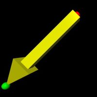
Vectors are visually represented by arrows. The length of the arrow represents the magnitude of the vector, while the direction the arrow points in represents the direction of the vector. If a vector exists at a particular point in space, the "tail" of the arrow (the end without the V shape) should be placed at that point. If the magnitude of the vector has units of length, the length of the arrow should conform to the coordinate system; otherwise, the length of the arrow can be any value, as long as it is proportional to the magnitude of the vector when compared to other vectors of the same property.
This example shows a visual representation of the velocity vector of a ball. The ball is at the position (2,3) and has a velocity of 5m/s in the +x direction.
A Mathematical Model
Forms
The information necessary to describe a specific vector can be presented in several forms.
One form in which vectors can be expressed is magnitude and direction form. In this form, the magnitude and the direction of the vector are explicitly stated. The statement describing direction might be a cardinal direction (ex. "north"), a direction on a graph (ex. "the +x direction"), or an angle (ex. "210[math]\displaystyle{ ^\circ }[/math] from the x axis counterclockwise"), depending on the situation. Magnitude and direction form is often used in word problems because it is easy for humans to understand.
Another form in which vectors can be expressed is component form. In this form, the vector is divided into components, each representing a different coordinate direction. In 2D space, these are the x and y directions. In 3D space, these are the x, y, and z directions.
The following calculations can be performed on vectors:
Finding the Magnitude: [math]\displaystyle{ |\vec A| = \sqrt{x^2 + y^2 + z^2} }[/math]
Finding the Unit Vector: :[math]\displaystyle{ \hat{A} = \frac{\vec A}{|\vec A|} }[/math]
Dot Product: [math]\displaystyle{ |\vec A \cdot \vec B| = |\vec A| \ast |\vec B| \ast \cos\Theta }[/math]
Cross Product: [math]\displaystyle{ |\vec A \times \vec B| = |\vec A| \ast |\vec B| \ast \sin\Theta }[/math]
Adding Two Vectors: [math]\displaystyle{ \lt A_1,\ A_2,\ A_3 \gt + \lt B_1,\ B_2,\ B_3 \gt \ =\ \lt A_1 + B_1,\ A_2 + B_2,\ A_3 + B_3 \gt }[/math]
Multiplying Two Vectors: [math]\displaystyle{ \vec A \times \vec B = \lt A_1,\ A_2,\ A_3 \gt \times \lt B_1,\ B_2,\ B_3 \gt = \lt A_2 \ast B_3 - A_3 \ast B_2 \gt \ i\ +\ \lt A_1 \ast B_3 - A_3 \ast B_1 \gt \ j\ +\ \lt A_1 \ast B_2 - A_2 \ast B_1 \gt \ k }[/math]
Multiplying a vector and a scalar: [math]\displaystyle{ C\ \ast\ \lt A_1,\ A_2,\ A_3 \gt \ =\ \lt C \ast A_1,\ C \ast A_2,\ C \ast A_3 \gt }[/math]
[math]\displaystyle{ \vec A \cdot \vec B\ =\ \sum_{i=1}^n A_iB_i=A_1B_1+A_2B_2+\cdots+A_nB_n }[/math]
A Computational Model

VIDLE is an interactive editor for VPython, a programming language that is commonly used in Physics to create 3D displays and animations. It is also used to perform iterative calculations using fundamental principles. Codes on VIDLE are instructions for a computer to follow to make these calculations.
In VIDLE code, arrow objects usually represent vector components. Arrows can be defined by their position, axis, and color. Each part can be manipulated to achieve different results. The position and axis of arrows are vectors, so they can be scaled by multiplying by a scalar. Arrows are often used to represent relative position vectors, starting at position A and ending at position B or by finding the "final minus initial" (B-A) position vector. In the image, the relative position vector is of the tennis ball with respect to the baseball, so the arrow points from the baseball to the tennis ball. If a relative position vector is in the 3D-plane, three further arrows can be used to denote the x, y, and z components. The z component vector is referenced using the formula vectorname.z.
In Physics 2, you will learn that a vector always starts at a source and points to the observation location at which physical quantities such as the electric or magnetic fields need to be found. Furthermore, it is important to be able to calculate the magnitude and direction of a vector in 3D space. Here is an example of a VPython model that computationally calculates such values. The green arrow represents the position vector which starts from a proton (red ball) to the arbitrary observation location. Click 'Run' on the upper-left corner in order to display the model.
--Htaghian3 (talk) 01:54, 16 September 2018 (EDT)
Examples
Simple
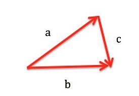
Which of the following statements is correct? (Can be more than one)

1. [math]\displaystyle{ \overrightarrow{c} = \overrightarrow{a} + \overrightarrow{b} }[/math]
2. [math]\displaystyle{ \overrightarrow{a} = \overrightarrow{b} - \overrightarrow{c} }[/math]
3. [math]\displaystyle{ \overrightarrow{a} = \overrightarrow{c} + \overrightarrow{b} }[/math]
4. [math]\displaystyle{ \overrightarrow{b} = \overrightarrow{c} + \overrightarrow{a} }[/math]
The answer is option number 2 and option number 4.
Intermediate
1. What is the magnitude of the vector C = A - B if A = <10, 5, 8> and B = <9, 4, 3>?
First we need to find the vector C: A - B = [math]\displaystyle{ \lt (10-9), (5-4), (8-3)\gt = \lt 1, 1, 5\gt = C }[/math]
[math]\displaystyle{ \sqrt{(1)^2 + 1^2 + 5^2} = 5.196 }[/math]
2. What is the cross product of A = <1,2,3> and B = <9,4,5>?
Use the equation for cross product: a x b= <a1, a2, a3> x <b1, b2, b3> = <a2*b3 - a3*b2> i - <a1*b3 - a3*b1> j + <a1*b2 - a2*b1> k
A x B[math]\displaystyle{ =\lt 2*5 - 3*4, 1*5 - 3*9, 1*4 - 2*9\gt = \lt -2, -22, -14\gt }[/math]
Difficult
What is the unit vector in the direction of the vector <10, 5, 8>? First you have to find the magnitude of the vector given: [math]\displaystyle{ \sqrt{10^2 + (5)^2 + 8^2} = 13.74 }[/math]
Finally divide the vector by its magnitude to get the unit vector:
[math]\displaystyle{ \tfrac{\lt 10, 5, 8\gt }{13.74} }[/math]
= <.727, .364, .582> Notice that the magnitude of the unit vector is equal to 1
Connectedness
1.Vectors will be used in many applications in most calculation based fields when movement and position are involved. Vectors can be two dimensional or three dimensional. Vectors are used to represent forces, fields, and momentum.
2.Vectors has been used in many application problems in engineering majors. In engineering applications, vectors are used to a lot of quantities which have both magnitude and direction. Dividing a magnitude into vector quantities in the x,y, and z directions clarify which components of a vector have quantity. For example, in Biomedical Engineering applications, vectors are used to represent the velocity of a flow to further calculate the flow rate and some other related quantities.
3. Vectors play a huge part in industry. For example, in process flow, vectors play a huge part in most calculations. For example, many calculations in different fields of science and math use vector components and direction. Our car's GPS uses vectors even if we don't realize it!
History
The discovery and use of vectors can date back to the ancient philosophers, Aristotle and Heron. The theory can also be found in the first article of Newtons Principia Mathematica. In the early 19th century Caspar Wessel, Jean Robert Argand, Carl Friedrich Gauss, and a few more depicted and worked with complex numbers as points on a 2D plane. in 1827, August Ferdinand published a book introducing line segments labelled with letters. he wrote about vectors without the name "vector".
In 1835, Giusto Bellavitis abstracted the basic idea of a vector while establishing the concept of equipollence. He called any pair of line segments of the same length and orientation equipollent (meaning equal length). He found a relationship and created the first set of vectors. Also in 1835 Hamilton founded "quaternions", which were 4D planes and equations with vectors.
William Rowan Hamilton devised the name "vector" as part of his system of quaternions consisting of three dimensional vectors.
Several other mathematicians developed similar vector systems to those of Bellavitis and Hamilton in the 19th century. The system used by Herman Grassman is the one that is most similar to the one used today.
VPython was released by David Scherer in the year 2000. He came up with the idea after taking a physics class at Carnegie Mellon University. Previous programs only allowed for 2D modeling, so he took it upon himself to make something better. VPython, also known as Visual Python, allows for 3D modeling.
See also
External links
Mathematical Computations on Vectors: [1]
Computational Work with Vectors: [2]
Basics of Vectors: [3]
Further Reading
Vector Analysis by Josiah Willard Gibbs
Introduction to Matrices and Vectors by Jacob T. Schwartz
