Iterative Prediction: Difference between revisions
| Line 70: | Line 70: | ||
===Example #1 - Momentum Update=== | ===Example #1 - Momentum Update=== | ||
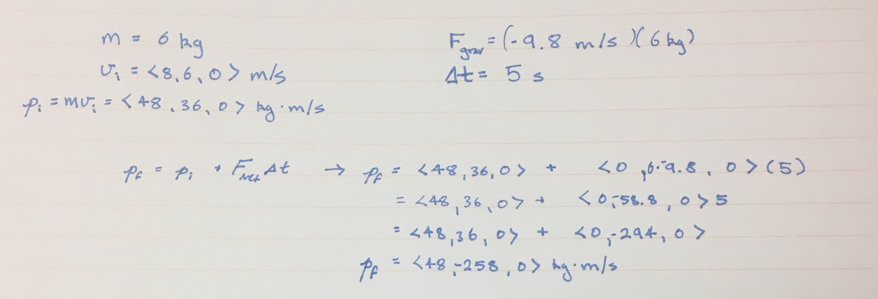
'''A 6kg ball is thrown into the air with an initial velocity of <math>{<8,6,0> m/s}</math>. If the only force acting on the ball is gravity, what is the final momentum of the ball after 5 seconds?''' | '''A 6kg ball is thrown into the air with an initial velocity of <math>{<8,6,0> m/s}</math>. If the only force acting on the ball is gravity, what is the final momentum of the ball after 5 seconds?''' | ||
[[File:EasyIterative.jpg | [[File:EasyIterative.jpg] | ||
===Example #2 - Trajectory Maxima=== | ===Example #2 - Trajectory Maxima=== | ||
Revision as of 23:31, 27 November 2016
JENNIFER YU (FALL 2016)
What is Iterative Prediction?
Iterative Prediction - a process used to predict the effects of a force (constant or varying), on the motion of an object over a specific time interval that is split up into many smaller intervals.
During each time interval (∆t):
         • The force acting on the object is found
         • Using the net force (Fnet), calculate the change of momentum (∆p) of the object
         • Using Fnet and ∆p, calculate the change in position of the object
         • Repeat this process for each new time interval.
Mathematical Explanation
         • Fnet = "some number"
         • ∆p = Fnet*∆t
         • ∆r = (v)*∆t
NOTE: The velocity used in the position update equation is the new velocity! Always use the velocity calculated from the final momentum in the previous step. [(p final /m object) = v]
Why do we use Iterative Prediction?
Iterative Prediction is a necessary technique to employ when doing physics because, even though our fundamental principles are based on calculus and derivatives and you should be able to solve these problems using integrals, it is often impossible to solve the integrals required to solve complex problems. Iterative Prediction also becomes much more convenient when you implement it using a program, such as vPython, which allows you to make the approximation use as many steps as your processing power can handle, which can make your prediction much more accurate.
A Mathematical Model
By starting from the general equation for the Momentum Principle, a formula can derived to predict the momentum of a given system at a specified point in the future. This is often referred to as the momentum update form of the Momentum Principle:
(1) [math]\displaystyle{ {\frac{∆\vec{p}}{dt}}_{system} = \vec{F}_{net} }[/math]
A system's change in momentum is equal to the net force acting on it over a specific interval of time.
(2) [math]\displaystyle{ {\vec{p}_{f} - \vec{p}_{i} = \vec{F}_{net}{Δt}} }[/math]
∆ stands for final minus initial. In this case, it's the system's final momentum minus its initial momentum that results in the overall change in momentum of the system.
(3) [math]\displaystyle{ {\vec{p}_{f} = \vec{p}_{i} + \vec{F}_{net}{Δt}} }[/math]
By adding the initial momentum value to the other side of the equation, it is now possible to solve for value of the system's final momentum.
Generally, the third form of the momentum principle is the most commonly used form in updating the momentum of a system. Due to the nature of iterative prediction (over many small intervals), any aspect of the equation can be "non-uniform" and still give calculable results.
To find the velocity used in the Position Update Formula, use the "final momentum" from the Momentum Update Equation to solve for the final velocity.
[math]\displaystyle{ {\frac{\vec{p}_{f}}m = \vec{v_{avg}}} }[/math]
Position Update Formula: [math]\displaystyle{ {\vec{r}_{f} = \vec{r}_{i} + \vec{v}_{avg}{Δt}} }[/math]
Remember: This process is repeated for EACH time interval that you are solving for/in.
A Visual Model
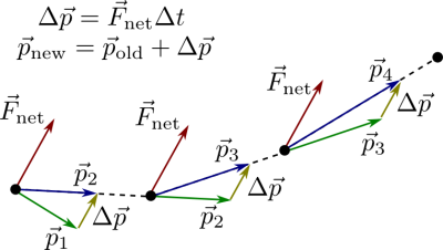
As seen from the Momentum Update Formula, the final momentum ([math]\displaystyle{ \vec{p}_{future} }[/math]) of a system after a given ∆t should be the sum of the initial momentum ([math]\displaystyle{ \vec{p}_{now} }[/math]) and the net force on the system multiplied by the ∆t. ([math]\displaystyle{ \vec{F}_{net}{Δt} }[/math]).

Each "step" in the diagram is a time interval in which the object's position and momentum was calculated for. This diagram also illustrates the explanation that having more intervals results in more accurate results (If you have more "steps" you'll have a more defined curve rather than a staircase like curve).
You can observe this Iterative Prediction in action by viewing this Vpython Script[1] (http://www.glowscript.org/#/user/JBarua/folder/Public/program/ProjectilePublic). It shows the flight path of a ball given an initial positive x and y velocity until it hits the ground, calculated using Iterative Prediction. In order to get a visual cue on how changing the time step of an Iterative Prediction calculation, try changing the deltat value from .15 to .05. You will see that making deltat smaller will place the approximation points closer together, which will give the ball's flight path a more consistent curve.
Example Calculations
There are a variety of different problems that can be solved by utilizing the momentum update form of the Momentum Principle. They can vary in difficulty and require any number of iterations. It is often prudent to calculate these iterations in a program loop to save time and avoid miscalculations.
Example #1 - Momentum Update
A 6kg ball is thrown into the air with an initial velocity of [math]\displaystyle{ {\lt 8,6,0\gt m/s} }[/math]. If the only force acting on the ball is gravity, what is the final momentum of the ball after 5 seconds? [[File:EasyIterative.jpg]
Example #2 - Trajectory Maxima
A 6kg ball is thrown into the air with an initial velocity of [math]\displaystyle{ {\lt 8,6,0\gt m/s} }[/math] and the only force acting on the ball is gravity. What is it's position after 5 seconds if it started out at [math]\displaystyle{ {\lt 3, 0 ,0\gt m} }[/math]

Example #3 - Varying Force
Connectedness
Iterative prediction is interesting to me in that modeling it's motion on a computer can be both complex and very simple. The idea that with a powerful processor you can get infinitely more accurate results than on a laptop is amazing. How much more accurate would our VPython be in lab? Does this mean that our VPython models are erroneous by miniscule amount? Beyond the process of answers, the idea that we are essentially "predicting the future" through math is exciting and really opens up a lot of questions as to the limit of what is predictable and what is not. The most simple idea resulting from iterative prediction is the principle of "this is where I started from, what will it take to get to here" or "this is where I started, where will I end up if I". As a biochemistry major, this principle is a large part of my laboratory procedures. Each reaction that I have to create isn't a blind "let's put in this much of reactant A with B and see how much C I end up with". It's always a question of calculating how much reactant is needed to complete the first reaction, as well calculating the results of what the product will be if this much reactant is added. For complex multi-step reactions, it's identical to the momentum update principle in that you are constantly taking what you are given and solving for where you end up after each reaction to get to the expected final product. Iterative prediction would be useful in pharmaceutical companies that are always trying to determine the effects of medications at the first instance of ingestion, and as the medicine dissolves (several reactions) in the stomach. Essentially, they would be creating multi-step reactions to simulate the human stomach in order to determine if the medication was performing as it should/not being detrimental towards our bodies.
History
The physics behind iterative prediction is nothing more than simple application of the momentum principle and projectile motion, which has existed in classical mechanics for quite some time. However, the practical application of iterative prediction for analyzing systems has evolved due to advances in computational methods and technology. With the computational power of a computer to iteratively calculate changes in momentum through time, one can analyze a system's motion extremely quickly without tedious and difficult mathematical calculations.
See also
There are many public resources that delve further into iterative prediction examples of more complex motion.
External links
MIT Open Courseware Introductory Mechanics
Iterative Prediction with VPython
References
CHANGE LECTURE SLIDES Georgia Institute of Technology. Physics Department. PHYS 2211. Fall 2016. Wednesday, Week 2 Lecture Slides. Fenton, Flavio H
Georgia Institute of Technology. Physics Department. PHYS 2211. Fall 2016. Monday, Week 3 Lecture Slides. Fenton, Flavio H
Georgia Institute of Technology. Physics Department. PHYS 2211. Fall 2016. Lab 07 Fancart Energy & Spring-Mass Instructions, Greco, Edwin
http://p3server.pa.msu.edu/coursewiki/doku.php?id=183_notes:iterativepredict